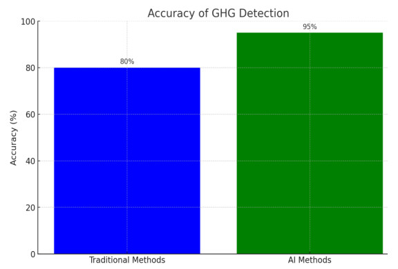
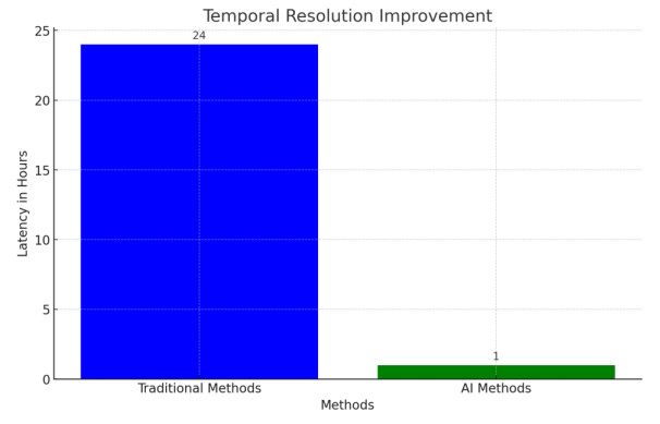
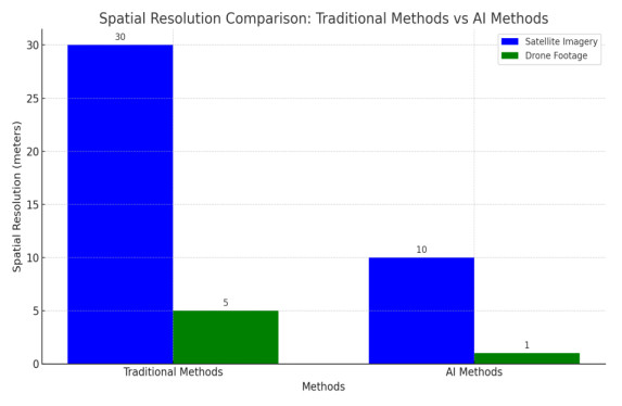
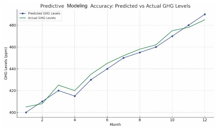
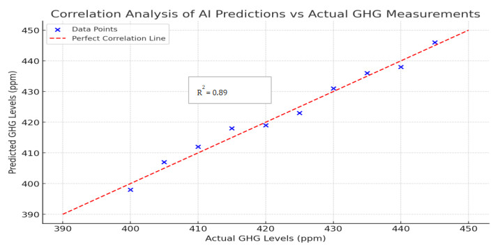
This research paper introduced a groundbreaking approach to greenhouse gas (GHG) monitoring by leveraging artificial intelligence (AI) technology to enhance both accuracy and efficiency. Traditional GHG monitoring methods are often hampered by high costs, labor-intensive processes, and significant delays in data analysis. This study harnessed advanced AI techniques, such as machine learning algorithms and neural networks, to facilitate real-time data collection and analysis from diverse sources including satellite imagery, Internet of Things (IoT) sensors, and atmospheric models. By implementing AI models like random forest, support vector machines, convolutional neural networks (CNNs), and long short-term memory (LSTM) networks, the research achieved substantial improvements such as reducing data reporting latency from 24 hours to just 1 hour, increasing spatial resolution from 30 meters to 10 meters, and enhancing detection accuracy from 80% to 95%. Additionally, the AI systems identified previously unknown emission sources and accurately forecasted future emission trends with a high correlation (R2 = 0.89). These advancements not only allow for more precise identification of emission hotspots and tracking of changes over time but also facilitate more effective regulatory responses and policy-making. The findings underscore the transformative potential of AI-driven monitoring systems in bolstering global sustainability efforts and combating climate change.
Citation: Rakibul Hasan, Rabeya Khatoon, Jahanara Akter, Nur Mohammad, Md Kamruzzaman, Atia Shahana, Sanchita Saha. AI-Driven greenhouse gas monitoring: enhancing accuracy, efficiency, and real-time emissions tracking[J]. AIMS Environmental Science, 2025, 12(3): 495-525. doi: 10.3934/environsci.2025023
This research paper introduced a groundbreaking approach to greenhouse gas (GHG) monitoring by leveraging artificial intelligence (AI) technology to enhance both accuracy and efficiency. Traditional GHG monitoring methods are often hampered by high costs, labor-intensive processes, and significant delays in data analysis. This study harnessed advanced AI techniques, such as machine learning algorithms and neural networks, to facilitate real-time data collection and analysis from diverse sources including satellite imagery, Internet of Things (IoT) sensors, and atmospheric models. By implementing AI models like random forest, support vector machines, convolutional neural networks (CNNs), and long short-term memory (LSTM) networks, the research achieved substantial improvements such as reducing data reporting latency from 24 hours to just 1 hour, increasing spatial resolution from 30 meters to 10 meters, and enhancing detection accuracy from 80% to 95%. Additionally, the AI systems identified previously unknown emission sources and accurately forecasted future emission trends with a high correlation (R2 = 0.89). These advancements not only allow for more precise identification of emission hotspots and tracking of changes over time but also facilitate more effective regulatory responses and policy-making. The findings underscore the transformative potential of AI-driven monitoring systems in bolstering global sustainability efforts and combating climate change.

| [1] |
Ahmed M, Ahmad I, Habibi D (2015) Green wireless-optical broadband access network: Energy and quality-of-service considerations. J Opt Commun Netw 7: 669–680. https://doi.org/10.1364/JOCN.7.000669 doi: 10.1364/JOCN.7.000669

|
| [2] | Al-Ajmai F F, Al-Otaibi F A, Aldaihani H M (2018) Effect of type of ground cover on the ground cooling potential for buildings in extreme desert climate. Jordan J Civ Eng 12. |
| [3] |
Sobuz M H R, Saleh M A, Samiun M, et al. (2025) AI-driven Modeling for the Optimization of Concrete Strength for Low-Cost Business Production in the USA Construction Industry. Eng Technol Appl Sci Res 15: 20529–20537. https://doi.org/10.48084/etasr.9733 doi: 10.48084/etasr.9733
|
| [4] |
Lorincz J, Garma T, Petrovic G (2012) Measurements and modelling of base station power consumption under real traffic loads. Sensors 12: 4281–4310. https://doi.org/10.3390/s120404281 doi: 10.3390/s120404281
|
| [5] |
Mishra M, Das D, Laurinavicius A, et al. (2025) Sectorial analysis of foreign direct investment and trade openness on carbon emissions: A threshold regression approach. J Int Commerce Econ Pol 16: 2550003. https://doi.org/10.1142/S1793993325500036 doi: 10.1142/S1793993325500036
|
| [6] |
Emre G, Akkus A, Karamış M B (2018) Wear resistance of Polymethyl Methacrylate (PMMA) with the Addition of Bone Ash, Hydroxylapatite and Keratin. IOP Conference Series: Materials Science and Engineering 295: 012004. https://doi.org/10.1088/1757-899X/295/1/012004 doi: 10.1088/1757-899X/295/1/012004
|
| [7] |
Chowhan S (2021) Potential Hazards of Air Pollution on Environment Health and Agriculture. Int J Environ Sci Nat Resour 28: 556231. https://doi.org/10.19080/IJESNR.2021.28.556231 doi: 10.19080/IJESNR.2021.28.556231
|
| [8] |
Gorgun E, Ali A, Islam M S (2024) Biocomposites of poly (lactic acid) and microcrystalline cellulose: influence of the coupling agent on thermomechanical and absorption characteristics. ACS Omega 9: 11523–11533. https://doi.org/10.1021/acsomega.3c08448 doi: 10.1021/acsomega.3c08448
|
| [9] |
Ahammad R, Hossain M K, Sobhan I, et al. (2023) Social-ecological and institutional factors affecting forest and landscape restoration in the Chittagong Hill Tracts of Bangladesh. Land Use Policy 125: 106478. https://doi.org/10.1016/j.landusepol.2022.106478 doi: 10.1016/j.landusepol.2022.106478
|
| [10] |
Al-Dahanii H, Watson P, Giles D (2015) Geotechnical and Geochemical Characterisation of Oil Fire Contaminated Soils in Kuwait. Eng Geol Soc Territ 6: 249–253. https://doi.org/10.1007/978-3-319-09060-3_40 doi: 10.1007/978-3-319-09060-3_40
|
| [11] |
Akkus A, Gorgun E (2015) The investigation of mechanical behaviors of poly methyl methacrylate (PMMA) with the addition of bone ash, hydroxyapatite and keratin. Adv Mater 4: 16–19. https://doi.org/10.11648/j.am.20150401.14 doi: 10.11648/j.am.20150401.14
|
| [12] |
Hasan R, Farabi S F, Kamruzzaman M, et al. (2024) AI-Driven Strategies for Reducing Deforestation. Am J Eng Technol 6: 6–20. https://doi.org/10.37547/tajet/Volume06Issue06-02 doi: 10.37547/tajet/Volume06Issue06-02
|
| [13] | Yoro K O, Daramola M O (2020) Chapter 1 - CO2 emission sources, greenhouse gases, and the global warming effect. Adv Carbon Capture 3–28. https://doi.org/10.1016/B978-0-12-819657-1.00001-3 |
| [14] |
Sobuz M H R, Datta S D, Jabin J A, et al. (2024) Assessing the influence of sugarcane bagasse ash for the production of eco-friendly concrete: Experimental and machine learning approaches. Case Stud Constr Mater 20: e02839., https://doi.org/10.1016/j.cscm.2023.e02839 doi: 10.1016/j.cscm.2023.e02839
|
| [15] |
Shang K, Xu L, Liu X, et al. (2023) Study of Urban Heat Island Effect in Hangzhou Metropolitan Area Based on SW-TES Algorithm and Image Dichotomous Model. Sage Open 13: 21582440231208851. https://doi.org/10.1177/21582440231208851 doi: 10.1177/21582440231208851
|
| [16] | Alsaffar A K K, Alquzweeni S S, Al-Ameer L R, et al. (2023) Development of eco-friendly wall insulation layer utilising the wastes of the packing industry, " Heliyon 9: e21799. https://doi.org/10.1016/j.heliyon.2023.e21799 |
| [17] |
Mishra M, Keshavarzzadeh V, Noshadravan A (2019) Reliability-based lifecycle management for corroding pipelines. Struct Saf 76: 1–14. https://doi.org/10.1016/j.strusafe.2018.06.007 doi: 10.1016/j.strusafe.2018.06.007
|
| [18] | Ibrahim A A, Kpochi K P, Smith E J (2018) Energy consumption assessment of mobile cellular networks. Am J Eng Res (AJER) 7: 96–101. |
| [19] |
Al-Otaibi F O, Aldaihani H M (2021) Experimental Investigation of the Applicability of Bitumen Stabilized Sabkha Soil as Landfill Liner in Kuwait. Int Rev Civil Eng 12: 298–304. https://doi.org/10.15866/irece.v12i5.18637 doi: 10.15866/irece.v12i5.18637
|
| [20] | Khirallah C, Thompson J S (2012) Energy efficiency of heterogeneous networks in lte-advanced. Journal of Signal Processing Systems. 69: 105-113. |
| [21] | Şenol H, Erşan M, Görgün E (2020) Biogas production from the co-digestion of urban solid waste and cattle manure. Avrupa Bilim ve Teknoloji Dergisi 396–403. |
| [22] | Villoria N, Garrett R, Gollnow F, et al. (2022) Leakage does not fully offset soy supply-chain efforts to reduce deforestation in Brazil. Nature Communications 13: 5476. |
| [23] | Yin Z, Liu Z, Liu X, et al. (2023) Urban heat islands and their effects on thermal comfort in the US: New York and New Jersey. Ecological Indicators 154: 110765. |
| [24] | Gorgun E (2024) Ultrasonic testing and surface conditioning techniques for enhanced thermoplastic adhesive bonds. J Mech Sci Technol 38: 1227-1236. |
| [25] | Şenol H, Oyan M, Görgün E (2024) Increasing the biomethane yield of hazelnut by-products by low temperature thermal pretreatment. Süleyman Demirel University Faculty of Arts and Science Journal of Science. 19: 18-28. |
| [26] |
Görgün E (2024) Investigation of The Effect of SMAW Parameters On Properties of AH36 Joints And The Chemical Composition of Seawater. Int J Innov Eng Appl 8: 28–36. https://doi.org/10.46460/ijiea.1418641 doi: 10.46460/ijiea.1418641
|
| [27] |
Akter J, Nilima S I, Hasan R, et al. (2024) Artificial intelligence on the agro-industry in the United States of America. AIMS Agri Food 9: 959–979. https://doi.org/10.3934/agrfood.2024052 doi: 10.3934/agrfood.2024052
|
| [28] |
Zhang T, Zhang W, Yang R, et al. (2021) CO2 capture and storage monitoring based on remote sensing techniques: A review. J Clean Prod 281: 124409. https://doi.org/10.1016/j.jclepro.2020.124409 doi: 10.1016/j.jclepro.2020.124409
|
| [29] |
Sun Y, Yin H, Wang W, et al. (2022) Monitoring greenhouse gases (GHGs) in China: status and perspective. Atmo Meas Tech 15: 4819–4834. https://doi.org/10.5194/amt-15-4819-2022 doi: 10.5194/amt-15-4819-2022
|
| [30] |
Filonchyk M, Yan H (2019) Urban air pollution monitoring by ground-based stations and satellite data. Springer 10: 978–3. https://doi.org/10.1007/978-3-319-78045-0 doi: 10.1007/978-3-319-78045-0
|
| [31] |
Şenol H, Çakır İ T, Bianco F, et al. (2024) Improved methane production from ultrasonically-pretreated secondary sedimentation tank sludge and new model proposal: Time series (ARIMA). Bioresour Technol 391: 129866. https://doi.org/10.1016/j.biortech.2023.129866 doi: 10.1016/j.biortech.2023.129866
|
| [32] |
Pan G, Xu Y, Ma J (2021) The potential of CO2 satellite monitoring for climate governance: A review. J Environ Manage 277: 111423. https://doi.org/10.1016/j.jenvman.2020.111423 doi: 10.1016/j.jenvman.2020.111423
|
| [33] |
Buchwitz M, Reuter M, Schneising O, et al. (2015) The Greenhouse Gas Climate Change Initiative (GHG-CCI): Comparison and quality assessment of near-surface-sensitive satellite-derived CO2 and CH4 global data sets. Remote Sens Environ 162: 344–362. https://doi.org/10.1016/j.rse.2013.04.024 doi: 10.1016/j.rse.2013.04.024
|
| [34] | Albergel E (2021) Earth observation satellites: Monitoring greenhouse gas emissions under the Paris Agreement. 2021. |
| [35] | Yu W, Hayat K, Ma J, et al. (2024) Effect of antibiotic perturbation on nitrous oxide emissions: An in-depth analysis. Crit Rev Environ Sci Technol 54: 1–21, |
| [36] |
Bibri S E, Krogstie J, Kaboli A, et al. (2024) Smarter eco-cities and their leading-edge artificial intelligence of things solutions for environmental sustainability: A comprehensive systematic review. Environ Sci Ecotechnol 19: 100330. https://doi.org/10.1016/j.ese.2023.100330 doi: 10.1016/j.ese.2023.100330
|
| [37] | Gaur L, Afaq A, Arora G K, et al. (2023) Artificial intelligence for carbon emissions using system of systems theory. Ecol Inform 76: 102165. https://doi.org/10.1016/j.ecoinf.2023.102165 |
| [38] | Cowls J, Tsamados A, Taddeo M, et al. (2023) The AI gambit: leveraging artificial intelligence to combat climate change—opportunities, challenges, and recommendations. Ai Society 2023: 1–25. |
| [39] |
Bottou L, Curtis F E, Nocedal J (2018) Optimization methods for large-scale machine learning. SIAM review 60: 223–311. https://doi.org/10.1137/16M1080173 doi: 10.1137/16M1080173
|
| [40] | Mishra M (2024) Quantifying compressive strength in limestone powder incorporated concrete with incorporating various machine learning algorithms with SHAP analysis. Asian J Civil Eng 26: 731–746. |
| [41] |
Görgün E (2022) Characterization of Superalloys by Artificial Neural Network Method. New Trends in Math Sci 2022: 67. https://doi.org/10.20852/ntmsci.2022.470 doi: 10.20852/ntmsci.2022.470
|
| [42] |
Jabin J A, Khondoker M T H, Sobuz M H R, et al. (2024) High-temperature effect on the mechanical behavior of recycled fiber-reinforced concrete containing volcanic pumice powder: An experimental assessment combined with machine learning (ML)-based prediction. Constr Build Mater 418: 135362. https://doi.org/10.1016/j.conbuildmat.2024.135362 doi: 10.1016/j.conbuildmat.2024.135362
|
| [43] |
Sobuz M H R, Joy L P, Akid A S M, et al. (2024) Optimization of recycled rubber self-compacting concrete: Experimental findings and machine learning-based evaluation. Heliyon 10: e27793. https://doi.org/10.1016/j.heliyon.2024.e27793 doi: 10.1016/j.heliyon.2024.e27793
|
| [44] |
Sobuz M H R, Aditto F S, Datta S D, et al. (2024) High-Strength Self-Compacting Concrete Production Incorporating Supplementary Cementitious Materials: Experimental Evaluations and Machine Learning Modelling. Int J Concr Struct Mater 18: 67. https://doi.org/10.1186/s40069-024-00707-7 doi: 10.1186/s40069-024-00707-7
|
| [45] |
Linkon A A, Noman I R, Islam M R, et al. (2024) Evaluation of Feature Transformation and Machine Learning Models on Early Detection of Diabetes Mellitus. IEEE Access 12: 165425–165440. https://doi.org/10.1109/ACCESS.2024.3488743 doi: 10.1109/ACCESS.2024.3488743
|
| [46] |
Hasan R, Biswas B, Samiun M, et al. (2025) Enhancing malware detection with feature selection and scaling techniques using machine learning models. Sci Rep 15: 9122. https://doi.org/10.1038/s41598-025-93447-x doi: 10.1038/s41598-025-93447-x
|
| [47] |
Lago J, De Ridder F, De Schutter B (2018) Forecasting spot electricity prices: Deep learning approaches and empirical comparison of traditional algorithms. Appl Energy 221: 386–405. https://doi.org/10.1016/j.apenergy.2018.02.069 doi: 10.1016/j.apenergy.2018.02.069
|
| [48] |
Sobuz M H R, Rahman M M, Aayaz R, et al. (2025) Combined influence of modified recycled concrete aggregate and metakaolin on high-strength concrete production: Experimental assessment and machine learning quantifications with advanced SHAP and PDP analyses. Constr Build Mater 461: 139897. https://doi.org/10.1016/j.conbuildmat.2025.139897 doi: 10.1016/j.conbuildmat.2025.139897
|
| [49] |
Schuh A E, Otte M, Lauvaux T, et al. (2021) Far-field biogenic and anthropogenic emissions as a dominant source of variability in local urban carbon budgets: A global high-resolution model study with implications for satellite remote sensing. Remote Sens Environ 262: 112473. https://doi.org/10.1016/j.rse.2021.112473 doi: 10.1016/j.rse.2021.112473
|
| [50] |
Hsu A, Khoo W, Goyal N, et al. (2020) Next-generation digital ecosystem for climate data mining and knowledge discovery: a review of digital data collection technologies. Front big Data 3: 29. https://doi.org/10.3389/fdata.2020.00029 doi: 10.3389/fdata.2020.00029
|
| [51] |
Romijn E, De Sy V, Herold M, et al. (2018) Independent data for transparent monitoring of greenhouse gas emissions from the land use sector – What do stakeholders think and need? Environ Sci Policy 85: 101–112. https://doi.org/10.1016/j.envsci.2018.03.016 doi: 10.1016/j.envsci.2018.03.016
|
| [52] |
Wang J, Li Y, Bork E W, et al. (2021) Effects of grazing management on spatio-temporal heterogeneity of soil carbon and greenhouse gas emissions of grasslands and rangelands: Monitoring, assessment and scaling-up. J Clean Prod 288: 125737. https://doi.org/10.1016/j.jclepro.2020.125737 doi: 10.1016/j.jclepro.2020.125737
|
| [53] |
Masood A, Ahmad K (2021) A review on emerging artificial intelligence (AI) techniques for air pollution forecasting: Fundamentals, application and performance. J Clean Prod 322: 129072. https://doi.org/10.1016/j.jclepro.2021.129072 doi: 10.1016/j.jclepro.2021.129072
|
| [54] |
Somantri A, Surendro K (2024) Greenhouse gas emission reduction architecture in computer science: A systematic review. IEEE Access https://doi.org/10.1109/ACCESS.2024.3373786 doi: 10.1109/ACCESS.2024.3373786
|
| [55] |
Li F, Yigitcanlar T, Nepal M, et al. (2023) Machine learning and remote sensing integration for leveraging urban sustainability: A review and framework. Sust Cities Soc 96: 104653. https://doi.org/10.1016/j.scs.2023.104653 doi: 10.1016/j.scs.2023.104653
|
| [56] |
Dumont Le Brazidec J, Vanderbecken P, Farchi A, et al. (2024) Deep learning applied to CO 2 power plant emissions quantification using simulated satellite images. Geosci Model Dev 17: 1995–2014. https://doi.org/10.5194/gmd-17-1995-2024 doi: 10.5194/gmd-17-1995-2024
|
| [57] |
Zheng Y, Liu F, Hsieh H P (2013) U-air: When urban air quality inference meets big data. Proceedings of the 19th ACM SIGKDD international conference on Knowledge discovery and data mining 2013: 1436–1444. https://doi.org/10.1145/2487575.2488188 doi: 10.1145/2487575.2488188
|
| [58] |
Kumar P, Druckman A, Gallagher J, et al. (2019) The nexus between air pollution, green infrastructure and human health. Environ Int 133: 105181. https://doi.org/10.1016/j.envint.2019.105181 doi: 10.1016/j.envint.2019.105181
|
| [59] |
Smith K R, Frumkin H, Balakrishnan K, et al. (2013) Energy and human health. Annual Review of public health 34: 159–188. https://doi.org/10.1146/annurev-publhealth-031912-114404 doi: 10.1146/annurev-publhealth-031912-114404
|
| [60] |
Sujatha K, Bhavani N P G, Ponmagal R S (2017) Impact of NO x emissions on climate and monitoring using smart sensor technology. 2017 International Conference on Communication and Signal Processing (ICCSP) 2017: 0853–0856. https://doi.org/10.1109/ICCSP.2017.8286488 doi: 10.1109/ICCSP.2017.8286488
|
| [61] | Bonire G, Gbenga-Ilori A (2021) Towards artificial intelligence-based reduction of greenhouse gas emissions in the telecommunications industry. Scientific African 12: e00823. |
| [62] |
Yavari A, Mirza I B, Bagha H, et al. (2023) ArtEMon: Artificial Intelligence and Internet of Things Powered Greenhouse Gas Sensing for Real-Time Emissions Monitoring. Sensors 23: 7971. https://doi.org/10.3390/s23187971 doi: 10.3390/s23187971
|
| [63] |
Lee S, Tae S (2020) Development of a decision support model based on machine learning for applying greenhouse gas reduction technology. Sustainability 12: 3582. https://doi.org/10.3390/su12093582 doi: 10.3390/su12093582
|
| [64] |
Ntafalias A, Tsakanikas S, Skarvelis-Kazakos S, et al. (2022) Design and Implementation of an Interoperable Architecture for Integrating Building Legacy Systems into Scalable Energy Management Systems. Smart Cities 5: 1421–1440. https://doi.org/10.3390/smartcities5040073 doi: 10.3390/smartcities5040073
|
| [65] | Rüffer D, Hoehne F, Bühler J (2018) New digital metal-oxide (MOx) sensor platform. Sensors 18: 1052. |
| [66] | Kumar A, Kumar A, Kwoka M, et al. (2024) IoT-enabled surface-active Pd-anchored metal oxide chemiresistor for H2S gas detection. Sensor Actuat B: Chem 402: 135065. |
| [67] | Ketkar N, Moolayil J, Ketkar N, et al. (2021) Convolutional neural networks. Deep Learning with Python: Learn Best Practices of Deep Learning Models with PyTorch. 197–242. https://doi.org/10.1007/978-1-4842-5364-9_6 |
| [68] |
Bhatt D, Patel C, Talsania H, et al. (2021) CNN variants for computer vision: History, architecture, application, challenges and future scope. Electronics 10: 2470. https://doi.org/10.3390/electronics10202470 doi: 10.3390/electronics10202470
|
| [69] |
Gimpel H, Heger S, Wöhl M (2022) Sustainable behavior in motion: designing mobile eco-driving feedback information systems. Inf Technol Manag 23: 299–314. https://doi.org/10.1007/s10799-021-00352-6 doi: 10.1007/s10799-021-00352-6
|
| [70] |
Oruh J, Viriri S, Adegun A (2022) Long short-term memory recurrent neural network for automatic speech recognition. IEEE Access 10: 30069–30079. https://doi.org/10.1109/ACCESS.2022.3159339 doi: 10.1109/ACCESS.2022.3159339
|
| [71] |
Al-Selwi S M, Hassan M F, Abdulkadir S J, et al. (2023) LSTM inefficiency in long-term dependencies regression problems. J Adv Res Appl Sci Eng Technology 30: 16–31. https://doi.org/10.37934/araset.30.3.1631 doi: 10.37934/araset.30.3.1631
|
| [72] |
Alharbi H A, Aldossary M (2021) Energy-efficient edge-fog-cloud architecture for IoT-based smart agriculture environment. Ieee Access 9: 110480–110492. https://doi.org/10.1109/ACCESS.2021.3101397 doi: 10.1109/ACCESS.2021.3101397
|
| [73] |
Coomonte R, Lastres C, Feijóo C, et al. (2012) A simplified energy consumption model for fiber-based Next Generation Access Networks. Telemat Inform 29: 375–386. https://doi.org/10.1016/j.tele.2011.11.005 doi: 10.1016/j.tele.2011.11.005
|
| [74] |
Naeem M, Pareek U, Lee D C, et al. (2013) Estimation of distribution algorithm for resource allocation in green cooperative cognitive radio sensor networks. Sensors 13: 4884–4905. https://doi.org/10.3390/s130404884 doi: 10.3390/s130404884
|
| [75] |
Bouziane S E, Khadir M T, Dugdale J (2021) A collaborative predictive multi-agent system for forecasting carbon emissions related to energy consumption. Multiagent Grid Syst 17: 39–58. https://doi.org/10.3233/MGS-210342 doi: 10.3233/MGS-210342
|
| [76] |
Fu C, Zhou S, Zhang J, et al. (2022) Risk-Averse support vector classifier machine via moments penalization. Int J Mach Learn Cybern 13: 3341–3358. https://doi.org/10.1007/s13042-022-01598-4 doi: 10.1007/s13042-022-01598-4
|
| [77] |
Belgiu M, Drăguţ L (2016) Random forest in remote sensing: A review of applications and future directions. ISPRS J Photogramm Remote Sens 114: 24–31. https://doi.org/10.1016/j.isprsjprs.2016.01.011 doi: 10.1016/j.isprsjprs.2016.01.011
|
| [78] |
Prasad A M, Iverson L R, Liaw A (2006) Newer classification and regression tree techniques: bagging and random forests for ecological prediction. Ecosystems 9: 181–199. https://doi.org/10.1007/s10021-005-0054-1 doi: 10.1007/s10021-005-0054-1
|
Figures(8) / Tables(6)

Rakibul Hasan, Rabeya Khatoon, Jahanara Akter, Nur Mohammad, Md Kamruzzaman, Atia Shahana, Sanchita Saha. AI-Driven greenhouse gas monitoring: enhancing accuracy, efficiency, and real-time emissions tracking[J]. AIMS Environmental Science, 2025, 12(3): 495-525. doi: 10.3934/environsci.2025023


 DownLoad: