Analysis of short-term air quality monitoring data in a coastal area

Suwimon Kanchanasuta; Sirapong Sooktawee; Natthaya Bunplod; Aduldech Patpai; Nirun Piemyai; Ratchatawan Ketwang; Suwimon Kanchanasuta; Sirapong Sooktawee; Natthaya Bunplod; Aduldech Patpai; Nirun Piemyai; Ratchatawan Ketwang

doi:10.3934/environsci.2021033

AIMS Environmental Science

2021, Volume 8, Issue 6: 517-531. doi: 10.3934/environsci.2021033

Previous Article Next Article

Research article

Analysis of short-term air quality monitoring data in a coastal area

1.
Mahidol University, Faculty of Public Health, Department of Environmental Health Sciences, 420/1 Rajvithi Rd., Ratchathewi District, Bangkok 10400 Thailand
2.
Center of Excellence on Environmental Health and Toxicology, Bangkok, Thailand
3.
Environmental Research and Training Center, Department of Environmental Quality Promotion, Ministry of Natural Resources and Environment, Klong 5, Klongluang, Pathum Thani 12120, Thailand

Received: 11 August 2021 Accepted: 18 October 2021 Published: 21 October 2021

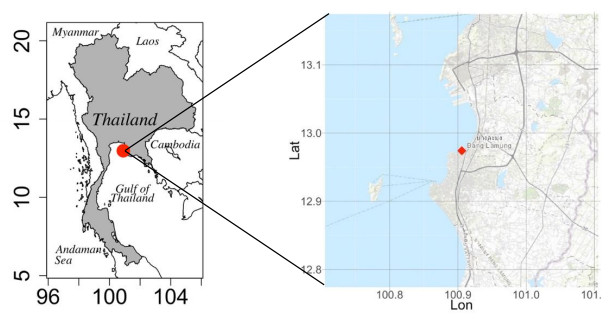
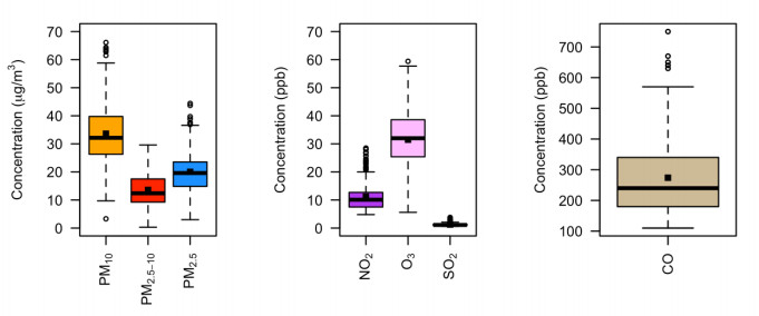
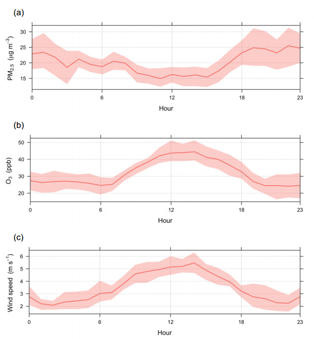
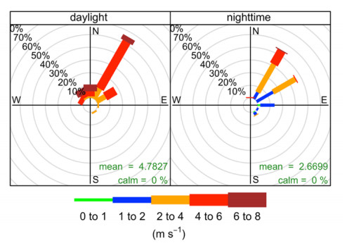
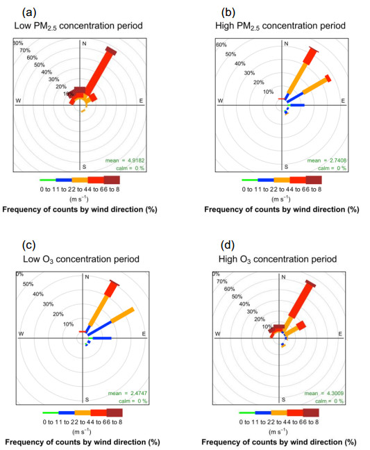
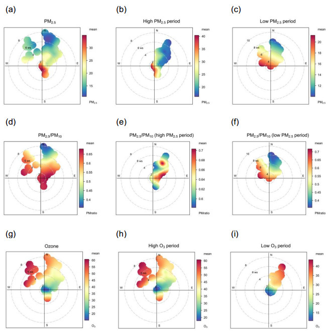
Short-term air quality monitoring in a coastal area, Naklua Subdistrict, Pattaya, Thailand is an activity to support the designated area under Thailand's sustainable tourism development. This study provided a short-term monitoring data analysis on time series and Bivariate Polar Plot (BVP) to provide the status of air quality and to determine the potential source area of air pollution. The result showed that NO₂, SO₂, CO and PM₁₀ were not higher than the national air quality standards, while the 24-hour average of PM_2.5 and the 8-hour average of O₃ were slightly higher than the World Health Organization (WHO) air quality guideline values. The nighttime PM_2.5 concentration was higher than the daytime concentration, and its potential source area is urban areas in the south. However, the daytime O₃ concentration is higher than the nighttime concentration. Its potential source area is from the northwest, where Sichang island is located. This result could be used to support air pollution management by controlling and reducing emissions in the potential source areas as the first priority. Also, the study revealed that the BVP technique could be used to determine the source area of air pollution in the coastal area, where wind circulation is more complex than that over the land.
- particulate matter,
- PM_2.5,
- ozone,
- O₃,
- air quality,
- bivariate polar plot,
- potential source area,
- coastal area,
- Thailand
Citation: Suwimon Kanchanasuta, Sirapong Sooktawee, Natthaya Bunplod, Aduldech Patpai, Nirun Piemyai, Ratchatawan Ketwang. Analysis of short-term air quality monitoring data in a coastal area[J]. AIMS Environmental Science, 2021, 8(6): 517-531. doi: 10.3934/environsci.2021033

Related Papers:

Abstract

Short-term air quality monitoring in a coastal area, Naklua Subdistrict, Pattaya, Thailand is an activity to support the designated area under Thailand's sustainable tourism development. This study provided a short-term monitoring data analysis on time series and Bivariate Polar Plot (BVP) to provide the status of air quality and to determine the potential source area of air pollution. The result showed that NO₂, SO₂, CO and PM₁₀ were not higher than the national air quality standards, while the 24-hour average of PM_2.5 and the 8-hour average of O₃ were slightly higher than the World Health Organization (WHO) air quality guideline values. The nighttime PM_2.5 concentration was higher than the daytime concentration, and its potential source area is urban areas in the south. However, the daytime O₃ concentration is higher than the nighttime concentration. Its potential source area is from the northwest, where Sichang island is located. This result could be used to support air pollution management by controlling and reducing emissions in the potential source areas as the first priority. Also, the study revealed that the BVP technique could be used to determine the source area of air pollution in the coastal area, where wind circulation is more complex than that over the land.

References

[1]	Janusz GK, Bajdor P (2013) Towards to Sustainable Tourism – Framework, Activities and Dimensions. Procedia Econ Finance 6: 523–529. doi: 10.1016/S2212-5671(13)00170-6
[2]	World Tourism Organization (Ed.) (2004) Indicators of sustainable development for tourism destinations: a guidebook, Madrid.
[3]	Sangkham S, Thongtip S, Vongruang P (2021) Influence of air pollution and meteorological factors on the spread of COVID-19 in the Bangkok Metropolitan Region and air quality during the outbreak. Environ Res 197: 111104. doi: 10.1016/j.envres.2021.111104
[4]	Darçın M (2014) Association between air quality and quality of life. Environ Sci Pollut Res 21: 1954–1959. doi: 10.1007/s11356-013-2101-3
[5]	Hopke PK (2016) Review of receptor modeling methods for source apportionment. J Air Waste Manag Assoc 66: 237–259. doi: 10.1080/10962247.2016.1140693
[6]	Grange SK, Lewis AC, Carslaw DC (2016) Source apportionment advances using polar plots of bivariate correlation and regression statistics. Atmos Environ 145: 128–134. doi: 10.1016/j.atmosenv.2016.09.016
[7]	Kanchanasuta S, Sooktawee S, Patpai A, et al. (2020) Temporal Variations and Potential Source Areas of Fine Particulate Matter in Bangkok, Thailand. Air Soil Water Res 13: 1–10. doi: 10.1177/1178622120978203
[8]	Sooktawee S, Kanchanasuta S, Boonyapitak S, et al. (2020) Distinguish Potential Source Areas of PM_2.5 and PM₁₀ by Statistical Data Analysis. IOP Conf Ser Earth Environ Sci 489: 012024. doi: 10.1088/1755-1315/489/1/012024
[9]	Sooktawee S, Kanabkaew T, Boonyapitak S, et al. (2020) Characterising particulate matter source contributions in the pollution control zone of mining and related industries using bivariate statistical techniques. Sci Rep 10: 21372. doi: 10.1038/s41598-020-78445-5
[10]	Uria-Tellaetxe I, Carslaw DC (2014) Conditional bivariate probability function for source identification. Environ Model Softw 59: 1–9. doi: 10.1016/j.envsoft.2014.05.002
[11]	Lu R, Turco RP (1994) Air Pollutant Transport in a Coastal Environment. Part I: Two-Dimensional Simulations of Sea-Breeze and Mountain Effects. J Atmospheric Sci 51: 2285–2308. doi: 10.1175/1520-0469(1994)051<2285:APTIAC>2.0.CO;2
[12]	Chirasophon S, Pochanart P (2020) The Long-term Characteristics of PM₁₀ and PM_2.5 in Bangkok, Thailand. Asian J Atmospheric Environ 14: 11. doi: 10.5572/ajae.2020.14.1.073
[13]	Wongsaming P, Exell RHB (2011) Criteria for Forecasting Cold Surges Associated with Strong High Pressure Areas over Thailand during the Winter Monsoon. J Sustain Energy Environ 2: 145–156.
[14]	Carslaw D, Beevers S, Ropkins K, et al. (2006) Detecting and quantifying aircraft and other on-airport contributions to ambient nitrogen oxides in the vicinity of a large international airport. Atmos Environ 40: 5424–5434. doi: 10.1016/j.atmosenv.2006.04.062
[15]	Carslaw DC, Ropkins K (2012) openair — An R package for air quality data analysis. Environ Model Softw 27–28: 52–61. doi: 10.1016/j.envsoft.2011.09.008
[16]	Carslaw DC, Beevers SD (2013) Characterising and understanding emission sources using bivariate polar plots and k-means clustering. Environ Model Softw 40: 325–329. doi: 10.1016/j.envsoft.2012.09.005
[17]	World Health Organization (Ed.) (2006) WHO Air quality guidelines for particulate matter, ozone, nitrogen dioxide and sulfur dioxide Global update 2005 Summary of risk assessment, Switzerland, World Health Organization.
[18]	Munir S (2017) Analysing Temporal Trends in the Ratios of PM_2.5/PM₁₀ in the UK. Aerosol Air Qual Res 17: 34–48. doi: 10.4209/aaqr.2016.02.0081
[19]	Seinfeld JH, Pandis SN (2006) Atmospheric chemistry and physics: from air pollution to climate change, Hoboken, N.J, J. Wiley.
[20]	Geiß A, Wiegner M, Bonn B, et al. (2017) Mixing layer height as an indicator for urban air quality? Atmospheric Meas Tech 10: 2969–2988. doi: 10.5194/amt-10-2969-2017
[21]	Guo J, Miao Y, Zhang Y, et al. (2016) The climatology of planetary boundary layer height in China derived fromradiosonde and reanalysis data. Atmospheric Chem Phys 16: 13309–13319. doi: 10.5194/acp-16-13309-2016
[22]	Liu S, Liang X-Z (2010) Observed Diurnal Cycle Climatology of Planetary Boundary Layer Height. J Clim 23: 5790–5809. doi: 10.1175/2010JCLI3552.1
[23]	Solanki R, Macatangay R, Sakulsupich V, et al. (2019) Mixing Layer Height Retrievals From MiniMPL Measurements in the Chiang Mai Valley: Implications for Particulate Matter Pollution. Front Earth Sci 7: 308. doi: 10.3389/feart.2019.00308
[24]	Nakoudi K, Giannakaki E, Dandou A, et al. (2019) Planetary boundary layer height by means of lidar and numerical simulations over New Delhi, India. Atmospheric Meas Tech 12: 2595–2610. doi: 10.5194/amt-12-2595-2019
[25]	Feng X, Wu B, Yan N (2015) A Method for Deriving the Boundary Layer Mixing Height from MODIS Atmospheric Profile Data. Atmosphere 6: 1346–1361. doi: 10.3390/atmos6091346
[26]	Sooktawee S, Humphries U, Limsakul A, et al. (2014) Spatio-Temporal Variability of Winter Monsoon over the Indochina Peninsula. Atmosphere 5: 101–121. doi: 10.3390/atmos5010101
[27]	Clarke A, Kapustin V, Howell S, et al. (2003) Sea-Salt Size Distributions from Breaking Waves: Implications for Marine Aerosol Production and Optical Extinction Measurements during SEAS. J Atmospheric Ocean Technol 20: 1362–1374. doi: 10.1175/1520-0426(2003)020<1362:SSDFBW>2.0.CO;2
[28]	Saliba G, Chen C-L, Lewis S, et al. (2019) Factors driving the seasonal and hourly variability of sea-spray aerosol number in the North Atlantic. Proc Natl Acad Sci 116: 20309–20314. doi: 10.1073/pnas.1907574116
[29]	Schiffer JM, Mael LE, Prather KA, et al. (2018) Sea Spray Aerosol: Where Marine Biology Meets Atmospheric Chemistry. ACS Cent Sci 4: 1617–1623. doi: 10.1021/acscentsci.8b00674
[30]	Zhao D, Chen H, Yu E, et al. (2019) PM_2.5/PM₁₀ Ratios in Eight Economic Regions and Their Relationship with Meteorology in China. Adv Meteorol 2019: 1–15.
[31]	Kleinman LI, Daum PH, Lee YN, et al. (2001) Sensitivity of ozone production rate to ozone precursors. Geophys Res Lett 28: 2903–2906. doi: 10.1029/2000GL012597
[32]	Reid N, Yap D, Bloxam R (2008) The potential role of background ozone on current and emerging air issues: An overview. Air Qual Atmosphere Health 1: 19–29. doi: 10.1007/s11869-008-0005-z
[33]	Awang NR, Ramli NA, Yahaya AS, et al. (2015) High Nighttime Ground-Level Ozone Concentrations in Kemaman: NO and NO₂ Concentrations Attributions. Aerosol Air Qual Res 15: 1357–1366. doi: 10.4209/aaqr.2015.01.0031
[34]	Velasco E, Rastan S (2015) Air quality in Singapore during the 2013 smoke-haze episode over the Strait of Malacca: Lessons learned. Sustain Cities Soc 17: 122–131. doi: 10.1016/j.scs.2015.04.006

Reader Comments

Your name:*

Email:*
© 2021 the Author(s), licensee AIMS Press. This is an open access article distributed under the terms of the Creative Commons Attribution License (http://creativecommons.org/licenses/by/4.0)