Patients with lesions in the posterior cingulate gyrus (PCG), including the retrosplenial cortex (RSC) and posterior cingulate cortex (PCC), cannot navigate in familiar environments, nor draw routes on a 2D map of the familiar environments. This suggests that the topographical knowledge of the environments (i.e., cognitive map) to find the right route to a goal is represented in the PCG, and the patients lack such knowledge. However, theoretical backgrounds in neuronal levels for these symptoms in primates are unclear. Recent behavioral studies suggest that human spatial knowledge is constructed based on a labeled graph that consists of topological connections (edges) between places (nodes), where local metric information, such as distances between nodes (edge weights) and angles between edges (node labels), are incorporated. We hypothesize that the population neural activity in the PCG may represent such knowledge based on a labeled graph to encode routes in both 3D environments and 2D maps. Since no previous data are available to test the hypothesis, we recorded PCG neuronal activity from a monkey during performance of virtual navigation and map drawing-like tasks. The results indicated that most PCG neurons responded differentially to spatial parameters of the environments, including the place, head direction, and reward delivery at specific reward areas. The labeled graph-based analyses of the data suggest that the population activity of the PCG neurons represents the distance traveled, locations, movement direction, and navigation routes in the 3D and 2D virtual environments. These results support the hypothesis and provide a neuronal basis for the labeled graph-based representation of a familiar environment, consistent with PCG functions inferred from the human clinicopathological studies.
Citation: Yang Yu, Tsuyoshi Setogawa, Jumpei Matsumoto, Hiroshi Nishimaru, Hisao Nishijo. Neural basis of topographical disorientation in the primate posterior cingulate gyrus based on a labeled graph[J]. AIMS Neuroscience, 2022, 9(3): 373-394. doi: 10.3934/Neuroscience.2022021
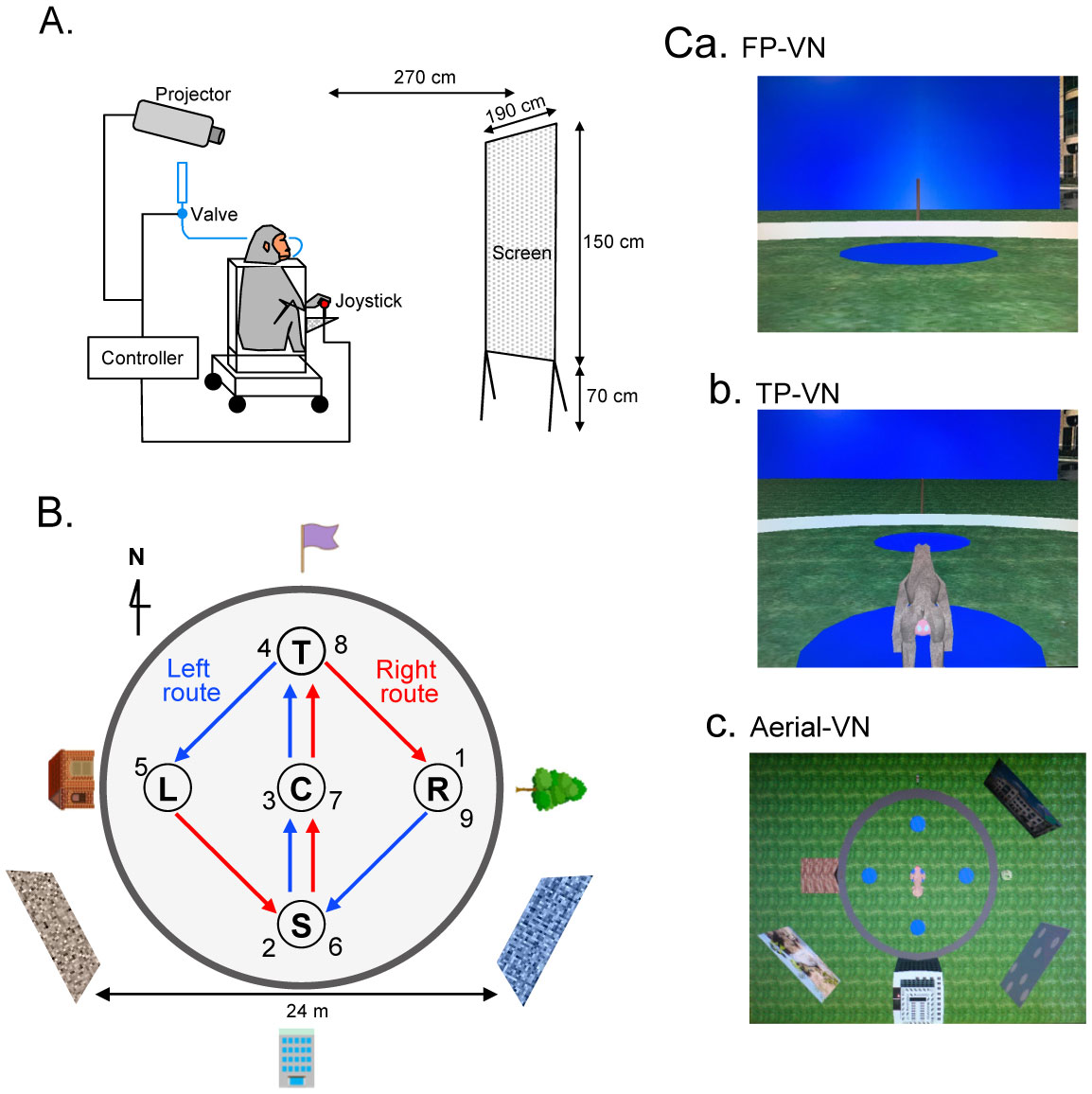
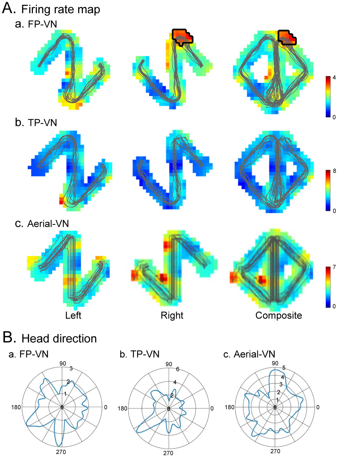
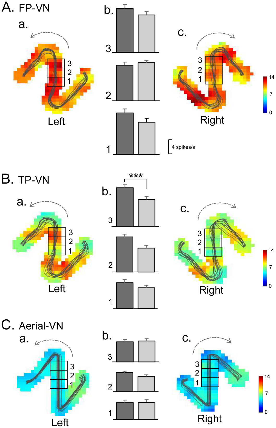
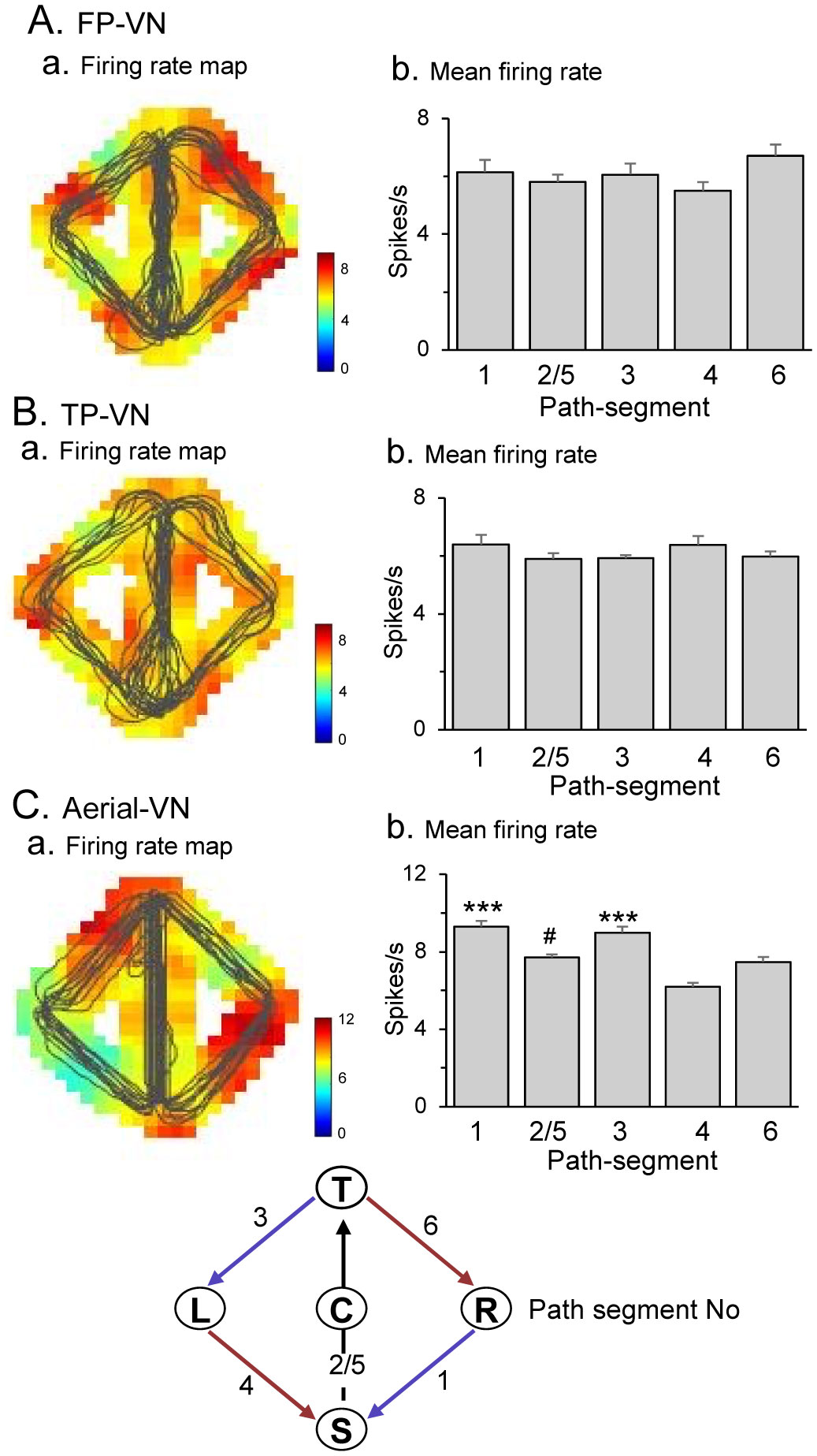
Patients with lesions in the posterior cingulate gyrus (PCG), including the retrosplenial cortex (RSC) and posterior cingulate cortex (PCC), cannot navigate in familiar environments, nor draw routes on a 2D map of the familiar environments. This suggests that the topographical knowledge of the environments (i.e., cognitive map) to find the right route to a goal is represented in the PCG, and the patients lack such knowledge. However, theoretical backgrounds in neuronal levels for these symptoms in primates are unclear. Recent behavioral studies suggest that human spatial knowledge is constructed based on a labeled graph that consists of topological connections (edges) between places (nodes), where local metric information, such as distances between nodes (edge weights) and angles between edges (node labels), are incorporated. We hypothesize that the population neural activity in the PCG may represent such knowledge based on a labeled graph to encode routes in both 3D environments and 2D maps. Since no previous data are available to test the hypothesis, we recorded PCG neuronal activity from a monkey during performance of virtual navigation and map drawing-like tasks. The results indicated that most PCG neurons responded differentially to spatial parameters of the environments, including the place, head direction, and reward delivery at specific reward areas. The labeled graph-based analyses of the data suggest that the population activity of the PCG neurons represents the distance traveled, locations, movement direction, and navigation routes in the 3D and 2D virtual environments. These results support the hypothesis and provide a neuronal basis for the labeled graph-based representation of a familiar environment, consistent with PCG functions inferred from the human clinicopathological studies.

| [1] |
Epstein RA (2008) Parahippocampal and retrosplenial contributions to human spatial navigation. Trends Cognitive Sci 12: 388-396. https://doi.org/10.1016/j.tics.2008.07.004 
|
| [2] |
Vann SD, Aggleton JP, Maguire EA (2009) What does the retrosplenial cortex do?. Nat Rev Neurosci 10: 792-802. https://doi.org/10.1038/nrn2733
|
| [3] |
Ghaem O, Mellet E, Crivello F, et al. (1997) Mental navigation along memorized routes activates the hippocampus, precuneus, and insula. Neuroreport 8: 739-744. https://doi.org/10.1097/00001756-199702100-00032
|
| [4] |
Maguire EA, Burgess N, Donnett JG, et al. (1998) Knowing where and getting there: a human navigation network. Science 280: 921-4. https://doi.org/10.1126/science.280.5365.921
|
| [5] |
Nemmi F, Piras F, Péran P, et al. (2013) Landmark sequencing and route knowledge: an fMRI study. Cortex 49: 507-19. https://doi.org/10.1016/j.cortex.2011.11.016
|
| [6] | Nguyen HM, Matsumoto J, Tran AH, et al. (2014) sLORETA current source density analysis of evoked potentials for spatial updating in a virtual navigation task. Front Behav Neurosci 8: 66. https://doi.org/10.3389/fnbeh.2014.00066 |
| [7] |
Patai EZ, Javadi AH, Ozubko JD, et al. (2019) Hippocampal and Retrosplenial Goal Distance Coding After Long-term Consolidation of a Real-World Environment. Cereb Cortex 29: 2748-2758. https://doi.org/10.1093/cercor/bhz044
|
| [8] |
Spiers HJ, Maguire EA (2006) Thoughts, behaviour, and brain dynamics during navigation in the real world. Neuroimage 31: 1826-40. https://doi.org/10.1016/j.neuroimage.2006.01.037
|
| [9] |
Brown TI, Carr VA, LaRocque KF, et al. (2016) Prospective representation of navigational goals in the human hippocampus. Science 352: 1323-6. https://doi.org/10.1126/science.aaf0784
|
| [10] |
Auger SD, Mullally SL, Maguire EA (2012) Retrosplenial cortex codes for permanent landmarks. PLoS One 7: e43620. https://doi.org/10.1371/journal.pone.0043620
|
| [11] |
Auger SD, Zeidman P, Maguire EA (2015) A central role for the retrosplenial cortex in de novo environmental learning. eLife 4: e09031. https://doi.org/10.7554/eLife.09031
|
| [12] |
Viard A, Doeller CF, Hartley T, et al. (2011) Anterior hippocampus and goal-directed spatial decision making. J Neurosci 31: 4613-21. https://doi.org/10.1523/JNEUROSCI.4640-10.2011
|
| [13] |
Takahashi N, Kawamura M, Shiota J, et al. (1997) Pure topographic disorientation due to right retrosplenial lesion. Neurology 49: 464-469. https://doi.org/10.1212/WNL.49.2.464
|
| [14] |
Aguirre GK, D'Esposito M (1999) Topographical disorientation: a synthesis and taxonomy. Brain 122: 1613-28. https://doi.org/10.1093/brain/122.9.1613
|
| [15] |
Vann SD, Aggleton JP (2002) Extensive cytotoxic lesions of the rat retrosplenial cortex reveal consistent deficits on tasks that tax allocentric spatial memory. Behav Neurosci 116: 85-94. https://doi.org/10.1037/0735-7044.116.1.85
|
| [16] |
Vann SD, Wilton LAK, Muir JL, et al. (2003) Testing the importance of the caudal retrosplenial cortex for spatial memory in rats. Behav Brain Res 140: 107-118. https://doi.org/10.1016/S0166-4328(02)00274-7
|
| [17] | Nelson AJ, Powell AL, Holmes JD, et al. (2015) What does spatial alternation tell us about retrosplenial cortex function. Front Behav Neurosci 9: 126. https://doi.org/10.3389/fnbeh.2015.00126 |
| [18] |
Chen LL, Lin LH, Barnes CA, et al. (1994a) Head-direction cells in the rat posterior cortex II. Contributions of visual and ideothetic information to the directional firing. Exp Brain Res 101: 24-34. https://doi.org/10.1007/BF00243213
|
| [19] |
Chen LL, Lin LH, Green EJ, et al. (1994b) Head-direction cells in the rat posterior cortex I. Anatomical distribution and behavioral modulation. Exp Brain Res 101: 8-23. https://doi.org/10.1007/BF00243212
|
| [20] |
Cho J, Sharp PE (2001) Head direction, place, and movement correlates for cells in the rat retrosplenial cortex. Behav Neurosci 115: 3-25. https://doi.org/10.1037/0735-7044.115.1.3
|
| [21] |
Jacob PY, Casali G, Spieser L, et al. (2017) An independent, landmark-dominated head-direction signal in dysgranular retrosplenial cortex. Nat Neurosci 20: 173-175. https://doi.org/10.1038/nn.4465
|
| [22] |
Chinzorig C, Nishimaru H, Matsumoto J, et al. (2020) Rat retrosplenial cortical involvement in wayfinding using visual and locomotor cues. Cereb Cortex 30: 1985-2004. https://doi.org/10.1093/cercor/bhz183
|
| [23] |
Fischer LF, Mojica Soto-Albors R, Buck F, et al. (2020) Representation of visual landmarks in retrosplenial cortex. Elife 9: e51458. https://doi.org/10.7554/eLife.51458
|
| [24] |
Alexander AS, Nitz DA (2015) Retrosplenial cortex maps the conjunction of internal and external spaces. Nat Neurosci 18: 1143-1151. https://doi.org/10.1038/nn.4058
|
| [25] |
Alexander AS, Nitz DA (2017) Spatially periodic activation patterns of retrosplenial cortex encode route sub-spaces and distance traveled. Curr Biol 27: 1551-1560. https://doi.org/10.1016/j.cub.2017.04.036
|
| [26] |
Miller AMP, Mau W, Smith DM (2019) Retrosplenial Cortical Representations of Space and Future Goal Locations Develop with Learning. Curr Biol 29: 2083-2090.e4. https://doi.org/10.1016/j.cub.2019.05.034
|
| [27] |
Dean HL, Platt ML (2006) Allocentric spatial referencing of neuronal activity in macaque posterior cingulate cortex. J Neurosci 26: 1117-1127. https://doi.org/10.1523/JNEUROSCI.2497-05.2006
|
| [28] |
Chrastil ER, Warren WH (2014) From cognitive maps to cognitive graphs. PLoS One 9: e112544. https://doi.org/10.1371/journal.pone.0112544
|
| [29] |
Muryy A, Glennerster A (2021) Route selection in non-Euclidean virtual environments. PLoS One 16: e0247818. https://doi.org/10.1371/journal.pone.0247818
|
| [30] |
Matsumura N, Nishijo H, Tamura R, et al. (1999) Spatial- and task-dependent neuronal responses during real and virtual translocation in the monkey hippocampal formation. J Neurosci 19: 2381-2393. https://doi.org/10.1523/JNEUROSCI.19-06-02381.1999
|
| [31] |
Hori E, Nishio Y, Kazui K, et al. (2005) Place-related neural responses in the monkey hippocampal formation in a virtual space. Hippocampus 15: 991-996. https://doi.org/10.1002/hipo.20108
|
| [32] |
Furuya Y, Matsumoto J, Hori E, et al. (2014) Place-related neuronal activity in the monkey parahippocampal gyrus and hippocampal formation during virtual navigation. Hippocampus 24: 113-130. https://doi.org/10.1002/hipo.22209
|
| [33] |
Bretas RV, Matsumoto J, Nishimaru H, et al. (2019) Neural Representation of Overlapping Path Segments and Reward Acquisitions in the Monkey Hippocampus. Front Syst Neurosci 13: 48. https://doi.org/10.3389/fnsys.2019.00048
|
| [34] |
Matsuda K (1996) Measurement system of the eye positions by using oval fitting of a pupil. Neurosci Res 25: S270-S270. https://doi.org/10.1016/0168-0102(96)89315-1
|
| [35] | Saleem KS, Logothetis NK (2012) A combined MRI and histology atlas of the rhesus monkey brain in stereotaxic coordinates. Waltham, Mass: Academic Press. |
| [36] |
Sun D, Unnithan RR, French C (2021b) Scopolamine Impairs Spatial Information Recorded With “Miniscope” Calcium Imaging in Hippocampal Place Cells. Front Neurosci 15: 640350. https://doi.org/10.3389/fnins.2021.640350
|
| [37] |
Mao D, Kandler S, McNaughton BL, et al. (2017) Sparse orthogonal population representation of spatial context in the retrosplenial cortex. Nat Commun 8: 243. https://doi.org/10.1038/s41467-017-00180-9
|
| [38] |
Sun W, Choi I, Stoyanov S, et al. (2021a) Context value updating and multidimensional neuronal encoding in the retrosplenial cortex. Nat Commun 12: 6045. https://doi.org/10.1038/s41467-021-26301-z
|
| [39] |
Liu B, Tian Q, Gu Y (2021) Robust vestibular self-motion signals in macaque posterior cingulate region. Elife 10: e64569. https://doi.org/10.7554/eLife.64569
|
| [40] |
Peer M, Ron Y, Monsa R, et al. (2019) Processing of different spatial scales in the human brain. Elife 8: e47492. https://doi.org/10.7554/eLife.47492
|
| [41] |
Peer M, Epstein RA (2021a) The human brain uses spatial schemas to represent segmented environments. Curr Biol 31: 4677-4688.e8. https://doi.org/10.1016/j.cub.2021.08.012
|
| [42] |
Enkhjargal N, Matsumoto J, Chinzorig C, et al. (2014) Rat thalamic neurons encode complex combinations of heading and movement directions and the trajectory route during translocation with sensory conflict. Front Behav Neurosci 8: 242. https://doi.org/10.3389/fnbeh.2014.00242
|
| [43] |
Frank LM, Brown EN, Wilson M (2000) Trajectory encoding in the hippocampus and entorhinal cortex. Neuron 27: 169-178. https://doi.org/10.1016/S0896-6273(00)00018-0
|
| [44] |
Wood ER, Dudchenko PA, Robitsek RJ, et al. (2000) Hippocampal neurons encode information about different types of memory episodes occurring in the same location. Neuron 27: 623-633. https://doi.org/10.1016/S0896-6273(00)00071-4
|
| [45] |
Ferbinteanu J, Shapiro ML (2003) Prospective and retrospective memory coding in the hippocampus. Neuron 40: 1227-1239. https://doi.org/10.1016/S0896-6273(03)00752-9
|
| [46] |
Dayawansa S, Kobayashi T, Hori E, et al. (2006) Conjunctive effects of reward and behavioral episodes on hippocampal place-differential neurons of rats on a mobile treadmill. Hippocampus 16: 586-595. https://doi.org/10.1002/hipo.20186
|
| [47] |
Sato N, Sakata H, Tanaka YL, et al. (2006) Navigation-associated medial parietal neurons in monkeys. Proc Natl Acad Sci U S A 103: 17001-17006. https://doi.org/10.1073/pnas.0604277103
|
| [48] | Vedder LC, Miller AMP, Harrison MB, et al. (2017) Retrosplenial cortical neurons encode navigational cues, trajectories and reward locations during goal directed navigation. Cereb Cortex 27: 3713-3723. https://doi.org/10.1093/cercor/bhw192 |
| [49] |
Franco LM, Goard MJ (2021) A distributed circuit for associating environmental context with motor choice in retrosplenial cortex. Sci Adv 7: eabf9815. https://doi.org/10.1126/sciadv.abf9815
|
| [50] | Zhang N, Grieves RM, Jeffery KJ (2021) Environment symmetry drives a multidirectional code in rat retrosplenial cortex. bioRxiv . https://doi.org/10.1101/2021.08.22.457261 |
| [51] |
Yan Y, Burgess N, Bicanski A (2021) A model of head direction and landmark coding in complex environments. PLoS Comput Biol 17: e1009434. https://doi.org/10.1371/journal.pcbi.1009434
|
| [52] |
Shinder ME, Taube JS (2011) Active and passive movement are encoded equally by head direction cells in the anterodorsal thalamus. J Neurophysiol 106: 788-800. https://doi.org/10.1152/jn.01098.2010
|
| [53] |
Vogt BA, Miller MW (1983) Cortical connections between rat cingulate cortex and visual, motor, and postsubicular cortices. J Comp Neurol 216: 192-210. https://doi.org/10.1002/cne.902160207
|
| [54] | Zilles K, Wree A (1995) Cortex: areal and laminar structure. The rat nervous system . San Diego, CA: Academic Press 649-685. |
| [55] |
Vogt BA, Vogt L, Laureys S (2006) Cytology and functionally correlated circuits of human posterior cingulate areas. Neuroimage 29: 452-466. https://doi.org/10.1016/j.neuroimage.2005.07.048
|
| [56] |
Rolls ET (2019) The cingulate cortex and limbic systems for emotion, action, and memory. Brain Struct Funct 224: 3001-3018. https://doi.org/10.1007/s00429-019-01945-2
|
| [57] |
Vann SD, Aggleton JP (2005) Selective dysgranular retrosplenial cortex lesions in rats disrupt allocentric performance of the radial-arm maze task. Behav Neurosci 119: 1682-1686. https://doi.org/10.1037/0735-7044.119.6.1682
|
| [58] |
Diekmann V, Jurgens R, Becker W (2009) Deriving angular displacement from optic flow: a fMRI study. Exp Brain Res 195: 101-116. https://doi.org/10.1007/s00221-009-1753-1
|
| [59] |
Huffman DJ, Ekstrom AD (2019) A Modality-Independent Network Underlies the Retrieval of Large-Scale Spatial Environments in the Human Brain. Neuron 104: 611-622.e7. https://doi.org/10.1016/j.neuron.2019.08.012
|
| [60] |
Burgess N, O'Keefe J (1996) Neuronal computations underlying the firing of place cells and their role in navigation. Hippocampus 6: 749-762. https://doi.org/10.1002/(SICI)1098-1063(1996)6:6<749::AID-HIPO16>3.0.CO;2-0
|
| [61] |
Poucet B, Hok V (2017) Remembering goal locations. Curr Opin Behav Sci 17: 51-56. https://doi.org/10.1016/j.cobeha.2017.06.003
|
| [62] |
Sarel A, Finkelstein A, Las L, et al. (2017) Vectorial representation of spatial goals in the hippocampus of bats. Science 355: 176-180. https://doi.org/10.1126/science.aak9589
|
| [63] |
Smith DM, Barredo J, Mizumori SJ (2012) Complimentary roles of the hippocampus and retrosplenial cortex in behavioral context discrimination. Hippocampus 22: 1121-1133. https://doi.org/10.1002/hipo.20958
|
| [64] |
Yoshida M, Chinzorig C, Matsumoto J, et al. (2021) Configural Cues Associated with Reward Elicit Theta Oscillations of Rat Retrosplenial Cortical Neurons Phase-Locked to LFP Theta Cycles. Cereb Cortex 31: 2729-2741. https://doi.org/10.1093/cercor/bhaa395
|
| [65] |
McCoy AN, Crowley JC, Haghighian G, et al. (2003) Saccade reward signals in posterior cingulate cortex. Neuron 40: 1031-1040. https://doi.org/10.1016/S0896-6273(03)00719-0
|
| [66] |
McCoy AN, Platt ML (2005) Risk-sensitive neurons in macaque posterior cingulate cortex. Nat Neurosci 8: 1220-1227. https://doi.org/10.1038/nn1523
|
| [67] |
Gauthier JL, Tank DW (2018) A dedicated population for reward coding in the hippocampus. Neuron 99: 179-193. https://doi.org/10.1016/j.neuron.2018.06.008
|
| [68] |
Dabaghian Y, Brandt VL, Frank LM (2014) Reconceiving the hippocampal map as a topological template. Elife 3: e03476. https://doi.org/10.7554/eLife.03476
|
| [69] |
Muller RU, Kubie JL, Saypoff R (1991) The hippocampus as a cognitive graph (abridged version). Hippocampus 1: 243-246. https://doi.org/10.1002/hipo.450010306
|
| [70] |
Trullier O, Wiener SI, Berthoz A, et al. (1997) Biologically based artificial navigation systems: review and prospects. Prog Neurobiol 51: 483-544. https://doi.org/10.1016/S0301-0082(96)00060-3
|
| [71] |
Peer M, Brunec IK, Newcombe NS, et al. (2021b) Structuring Knowledge with Cognitive Maps and Cognitive Graphs. Trends Cogn Sci 25: 37-54. https://doi.org/10.1016/j.tics.2020.10.004
|
| [72] |
Poucet B, Herrmann T (2001) Exploratory patterns of rats on a complex maze provide evidence for topological coding. Behav Processes 53: 155-162. https://doi.org/10.1016/S0376-6357(00)00151-0
|
| [73] |
Xu Z, Skorheim S, Tu M, et al. (2017) Improving efficiency in sparse learning with the feedforward inhibitory motif. Neurocomputing 267: 141-151. https://doi.org/10.1016/j.neucom.2017.05.016
|
| [74] |
Tukker JJ, Beed P, Brecht M, et al. (2022) Microcircuits for spatial coding in the medial entorhinal cortex. Physiol Rev 102: 653-688. https://doi.org/10.1152/physrev.00042.2020
|
| [75] |
Stacho M, Manahan-Vaughan D (2022) Mechanistic flexibility of the retrosplenial cortex enables its contribution to spatial cognition. Trends Neurosci 45: 284-296. https://doi.org/10.1016/j.tins.2022.01.007
|
| [76] |
Ison MJ, Mormann F, Cerf M, et al. (2011) Selectivity of pyramidal cells and interneurons in the human medial temporal lobe. J Neurophysiol 106: 1713-1721. https://doi.org/10.1152/jn.00576.2010
|
| [77] |
Dinh HT, Nishimaru H, Matsumoto J, et al. (2018) Superior Neuronal Detection of Snakes and Conspecific Faces in the Macaque Medial Prefrontal Cortex. Cereb Cortex 28: 2131-2145. https://doi.org/10.1093/cercor/bhx118
|
| [78] |
Sulpizio V, Committeri G, Lambrey S, et al. (2013) Selective role of lingual/parahippocampal gyrus and retrosplenial complex in spatial memory across viewpoint changes relative to the environmental reference frame. Behav Brain Res 242: 62-75. https://doi.org/10.1016/j.bbr.2012.12.031
|
| [79] |
Epstein RA, Vass LK (2013) Neural systems for landmark-based wayfinding in humans. Philos Trans R Soc Lond B Biol Sci 369: 20120533. https://doi.org/10.1098/rstb.2012.0533
|
| [80] |
Lambrey S, Doeller C, Berthoz A, et al. (2012) Imagining being somewhere else: neural basis of changing perspective in space. Cereb Cortex 22: 166-174. https://doi.org/10.1093/cercor/bhr101
|
| [81] |
Chrastil ER, Sherrill KR, Hasselmo ME, et al. (2015) There and Back Again: Hippocampus and Retrosplenial Cortex Track Homing Distance during Human Path Integration. J Neurosci 35: 15442-15452. https://doi.org/10.1523/JNEUROSCI.1209-15.2015
|
| [82] |
Chrastil ER, Sherrill KR, Aselcioglu I, et al. (2017) Individual Differences in Human Path Integration Abilities Correlate with Gray Matter Volume in Retrosplenial Cortex, Hippocampus, and Medial Prefrontal Cortex. eNeuro 4: ENEURO.0346-16.2017. https://doi.org/10.1523/ENEURO.0346-16.2017
|
| [83] |
Byrne P, Becker S, Burgess N (2007) Remembering the past and imagining the future: a neural model of spatial memory and imagery. Psychol Rev 114: 340-375. https://doi.org/10.1037/0033-295X.114.2.340
|
| [84] |
Chrastil ER (2013) Neural evidence supports a novel framework for spatial navigation. Psychon Bull Rev 20: 208-27. https://doi.org/10.3758/s13423-012-0351-6
|
| [85] |
Guterstam A, Björnsdotter M, Gentile G, et al. (2015) Posterior cingulate cortex integrates the senses of self-location and body ownership. Curr Biol 25: 1416–25. https://doi.org/10.1016/j.cub.2015.03.059
|
| [86] |
Hirshhorn M, Grady C, Rosenbaum RS, et al. (2012) Brain regions involved in the retrieval of spatial and episodic details associated with a familiar environment: an fMRI study. Neuropsychologia 50: 3094-106. https://doi.org/10.1016/j.neuropsychologia.2012.08.008
|
| [87] |
Ziv Y, Burns LD, Cocker ED, et al. (2013) Long-term dynamics of CA1 hippocampal place codes. Nat Neurosci 16: 264-266. https://doi.org/10.1038/nn.3329
|
| [88] |
Mao D, Neumann AR, Sun J, et al. (2018) Hippocampus-dependent emergence of spatial sequence coding in retrosplenial cortex. Proc Natl Acad Sci U S A 115: 8015-8018. https://doi.org/10.1073/pnas.1803224115
|
| [89] |
Steel A, Billings MM, Silson EH, et al. (2021) A network linking scene perception and spatial memory systems in posterior cerebral cortex. Nat Commun 12: 2632. https://doi.org/10.1038/s41467-021-22848-z
|
| [90] |
Papma JM, Smits M, de Groot M, et al. (2017) The effect of hippocampal function, volume and connectivity on posterior cingulate cortex functioning during episodic memory fMRI in mild cognitive impairment. Eur Radiol 27: 3716-3724. https://doi.org/10.1007/s00330-017-4768-1
|
| [91] |
Vanneste S, Luckey A, McLeod SL, et al. (2021) Impaired posterior cingulate cortex-parahippocampus connectivity is associated with episodic memory retrieval problems in amnestic mild cognitive impairment. Eur J Neurosci 53: 3125-3141. https://doi.org/10.1111/ejn.15189
|
 neurosci-09-03-021-s001.pdf neurosci-09-03-021-s001.pdf |
 |
Figures(7)

Yang Yu, Tsuyoshi Setogawa, Jumpei Matsumoto, Hiroshi Nishimaru, Hisao Nishijo. Neural basis of topographical disorientation in the primate posterior cingulate gyrus based on a labeled graph[J]. AIMS Neuroscience, 2022, 9(3): 373-394. doi: 10.3934/Neuroscience.2022021


 DownLoad: