Using dual-channel CNN to classify hyperspectral image based on spatial-spectral information

Haifeng Song; Weiwei Yang; Songsong Dai; Lei Du; Yongchen Sun; Haifeng Song; Weiwei Yang; Songsong Dai; Lei Du; Yongchen Sun

doi:10.3934/mbe.2020195

Mathematical Biosciences and Engineering

2020, Volume 17, Issue 4: 3450-3477. doi: 10.3934/mbe.2020195

Previous Article Next Article

Research article Special Issues

Using dual-channel CNN to classify hyperspectral image based on spatial-spectral information

1.
School of Electronics and Information Engineering (School of Big Data Science), Taizhou University, Taizhou, China
2.
The Transportation Monitoring and Emergency Response Center of Shandong Province, Jinan, China

Received: 23 January 2020 Accepted: 22 April 2020 Published: 05 May 2020

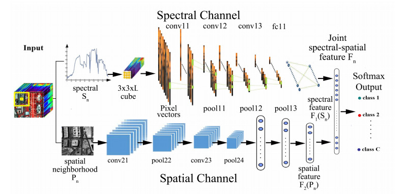
In the field of remote sensing image processing, the classification of hyperspectral image (HSI) is a hot topic. There are two main problems lead to the classification accuracy unsatisfactory. One problem is that the recent research on HSI classification is based on spectral features, the relationship between different pixels has been ignored; the other is that the HSI data does not contain or only contain a small amount of labeled data, so it is impossible to build a well classification model. To solve these problems, a dual-channel CNN model has been proposed to boost its discriminative capability for HSI classification. The proposed dual-channel CNN model has several distinct advantages. Firstly, the model consists of spectral feature extraction channel and spatial feature extraction channel; the 1-D CNN and 3-D CNN are used to extract the spectral and spatial features, respectively. Secondly, the dual-channel CNN have been used for fusing the spatial-spectral features, the fusion feature is input into the classifier, which effectively improves the classification accuracy. Finally, due to considering the spatial and spectral features, the model can effectively solve the problem of lack of training samples. The experiments on benchmark data sets have demonstrated that the proposed dual-channel CNN model considerably outperforms other state-of-the-art method.
- hyperspecral image,
- spatial-spectral information,
- dual-channel,
- convolutional neural network,
- classification
Citation: Haifeng Song, Weiwei Yang, Songsong Dai, Lei Du, Yongchen Sun. Using dual-channel CNN to classify hyperspectral image based on spatial-spectral information[J]. Mathematical Biosciences and Engineering, 2020, 17(4): 3450-3477. doi: 10.3934/mbe.2020195

Related Papers:

Abstract

In the field of remote sensing image processing, the classification of hyperspectral image (HSI) is a hot topic. There are two main problems lead to the classification accuracy unsatisfactory. One problem is that the recent research on HSI classification is based on spectral features, the relationship between different pixels has been ignored; the other is that the HSI data does not contain or only contain a small amount of labeled data, so it is impossible to build a well classification model. To solve these problems, a dual-channel CNN model has been proposed to boost its discriminative capability for HSI classification. The proposed dual-channel CNN model has several distinct advantages. Firstly, the model consists of spectral feature extraction channel and spatial feature extraction channel; the 1-D CNN and 3-D CNN are used to extract the spectral and spatial features, respectively. Secondly, the dual-channel CNN have been used for fusing the spatial-spectral features, the fusion feature is input into the classifier, which effectively improves the classification accuracy. Finally, due to considering the spatial and spectral features, the model can effectively solve the problem of lack of training samples. The experiments on benchmark data sets have demonstrated that the proposed dual-channel CNN model considerably outperforms other state-of-the-art method.

References

[1]	T. V. V Bandos, L. Bruzzone, G. Camps-Valls, Classification of hyperspectral images with regularized linear discriminant analysis, IEEE Trans. Geosci. Remote Sens., 47 (2009), 862-873.
[2]	G. Licciardi, P. R. Marpu, J. Chanussot, J. A. Benediktsson, Linear versus nonlinear PCA for the classification of hyperspectral data based on the extended morphological profiles, IEEE Geosci. Remote Sens. Lett., 9 (2012), 447-451. doi: 10.1109/LGRS.2011.2172185
[3]	A. Villa, J. A. Benediktsson, J. Chanussot, C. Jutten, Hyperspectral image classification with Independent component discriminant analysis, IEEE Transact. Geosci. Remote Sens., 49 (2011), 4865-4876. doi: 10.1109/TGRS.2011.2153861
[4]	H. Bischof, A. Leonardis, Finding optimal neural networks for land use classification, NIeee Trans. Geosci. Remote Sens., 36 (1998), 337-341. doi: 10.1109/36.655348
[5]	G. Camps-Valls, L. Gomez-Chova, J. Calpe-Maravilla, J. D. Martin-Guerrero, E. Soria-Olivas, L. Alonso-Chorda, et al., Robust support vector method for hyperspectral data classification and knowledge discovery, IEEE Trans. Geosci. Remote Sens., 42 (2004), 1-13.
[6]	D. L. Civco, Artificial neural networks for land-cover classification and mapping, Int. J. Geogr. Inf. Syst., 7 (1993), 173-186. doi: 10.1080/02693799308901949
[7]	F. Melgani, L. Bruzzone, Classification of hyperspectral remote sensing images with support vector machines, IEEE Trans. Geosci. Remote Sens., 42 (2004), 1778-1790. doi: 10.1109/TGRS.2004.831865
[8]	S. Haifeng, C. Guangsheng, W. Hairong, Y. Weiwei, The improved (2D)²PCA algorithm and its parallel implementation based on image block, Microprocess. Microsyst., 47 (2016), 170-177. doi: 10.1016/j.micpro.2016.06.011
[9]	Y. Chen, Z. Lin, X. Zhao, G. Wang, Y. Gu, Deep learning-based classification of hyperspectral data, IEEE J. Sel. Top. Appl. Earth Obs. Remote Sens., 7 (2014), 2094-2107. doi: 10.1109/JSTARS.2014.2329330
[10]	X. Chen, S. Xiang, C. L. Liu, C. H. Pan, Vehicle detection in satellite images by hybrid deep convolutional neural networks, IEEE Geosci. Remote Sens. Lett., 11 (2014), 1797-1801. doi: 10.1109/LGRS.2014.2309695
[11]	Z. Feng, S. Yang, S. Wang, L. Jiao Discriminative spectral-spatial margin-based semisupervised dimensionality reduction of hyperspectral data, IEEE Trans. Geosci. Remote Sens., 12 (2014), 224-228.
[12]	Z. Wang, N. M. Nasrabadi, T. S. Huang, Spatial-spectral classification of hyperspectral images using discriminative dictionary designed by learning vector quantization, IEEE Trans. Geosci. Remote Sens., 52 (2014), 4808-4822. doi: 10.1109/TGRS.2013.2285049
[13]	S. Bernabe, P. R. Marpu, A. Plaza, M. D. Mura, J. A. Benediktsson, Spectral-spatial classification of multispectral images using kernel feature space representation, IEEE Geosci. Remote Sens. Lett., 11 (2013), 228-292.
[14]	R. Ji, Y. Gao, R. Hong, Q. Liu, D. Tao, X. Li, Spectral-spatial constraint hyperspectral image classification, IEEE Trans. Geosci. Remote Sens., 3 (2014), 1811-1824.
[15]	M. Fauvel, Y. Tarabalka, J. A. Benediktsson, J. Chanussot, J. C. Tilton, Advances in spectralspatial classification of hyperspectral images, Proc. IEEE, 101 (2013), 652-675. doi: 10.1109/JPROC.2012.2197589
[16]	W. Zhao, S. Du, Spectral-spatial feature extraction for hyperspectral image classification: a dimension reduction and deep learning approach, IEEE Trans. Geosci. Remote Sens., 54 (2016), 4544-4554. doi: 10.1109/TGRS.2016.2543748
[17]	J. M. Bioucas-Dias, A. Plaza, G. Camps-Valls, P. Scheunders, N. M. Nasrabadi, J. Chanussot, Hyperspectral remote sensing data analysis and future challenges, IEEE Geosci. Remote Sens. Mag., 1 (2013), 6-36.
[18]	G. Camps-Valls, L. Gomez-Chova, J. Muñoz-Marí, J. Vila-Francés, J. Calpe-Maravilla, Composite kernels for hyperspectral image classification, IEEE Geosci. Remote Sens. Lett., 3 (2006), 93-97.
[19]	J. Li, P. R. Marpu, A. Plaza, J. M. Bioucas-Dias, J. A. Benediktsson, Generalized composite kernel framework for hyperspectral image classification, IEEE Trans. Geosci. Remote Sens., 51 (2013), 4816-4829. doi: 10.1109/TGRS.2012.2230268
[20]	Jun Li, José M. Bioucas-Dias, Antonio Plaza, Spectral-spatial classification of hyperspectral data using loopy belief propagation and active learning, IEEE Transact. Geosci. Remote Sens., 51 (2013), 844-856.
[21]	Z. Zhong, B. Fan, J. Duan, et al. Discriminant tensor spectral-spatial feature extraction for hyperspectral image classification, IEEE Geosci. Remote Sens. Lett., 12 (2015), 1028-1032. doi: 10.1109/LGRS.2014.2375188
[22]	X. Kang, S. Li, J. A. Benediktsson, Spectral-spatial hyperspectral image classification with edgepreserving filtering, IEEE Transact. Geosci. Remote Sens., 52 (2014), 2666-2677. doi: 10.1109/TGRS.2013.2264508
[23]	Y. Zhou, J. Peng, C. L. P. Chen, Dimension reduction using spatial and spectral regularized local discriminant embedding for hyperspectral image classification, IEEE Trans. Geosci. Remote Sens., 53 (2015), 1082-1095. doi: 10.1109/TGRS.2014.2333539
[24]	H. Zhang, Y. Li, Y. Zhang, Q. Shen, Spectral-spatial classification of hyperspectral imagery using a dual-channel convolutional neural network, Remote Sens. Lett., 8 (2017), 438-447. doi: 10.1080/2150704X.2017.1280200
[25]	Y. Chen, X. Zhao, X. Jia, Spectral-spatial classification of hyperspectral data based on deep belief network, IEEE J. Sel. Top. Appl. Earth Obs. Remote Sens., 8 (2015), 2381-2392. doi: 10.1109/JSTARS.2015.2388577
[26]	W. Hu, Y. Huang, L. Wei, F. Zhang, H. Li, Deep convolutional neural networks for hyperspectral image classification, J. Sensor., 2015 (2015), 1-12.
[27]	Z. Lin, Y. Chen, X. Zhao, G. Wang, Spectral-spatial classification of hyperspectral image using autoencoders, 2013 9th International Conference on Information, Communications & Signal Processing, Volume (2014).
[28]	P. Ghamisi, J. Plaza, Y. Chen, J. Li, A. J. Plaza, Advanced spectral classifiers for hyperspectral images: A review, IEEE Geosci. Remote Sens. Mag., 5 (2017), 8-32.
[29]	L. Zhang, L. Zhang, B. Du, Deep learning for remote sensing data: A technical tutorial on the state of the art, IEEE Geosci. Remote Sens. Mag., 4 (2016), 22-40. doi: 10.1109/MGRS.2016.2540798
[30]	Y. Lecun, Y. Bengio, G. Hinton, ImageNet classification with deep convolutional neural networks, Nature, 521 (2015), 436. doi: 10.1038/nature14539
[31]	W. Li, G. Wu, F. Zhang, Q. Du, Hyperspectral image classification using deep pixel-pair features, IEEE Transact. Geosci. Remote Sens., 55 (2017), 844-853. doi: 10.1109/TGRS.2016.2616355
[32]	W. Zhao, S. Du, Spectral-spatial feature extraction for hyperspectral image classification: A dimension reduction and deep learning approach, IEEE Transact. Geosci. Remote Sens., 54 (2016), 4544-4554. doi: 10.1109/TGRS.2016.2543748
[33]	Y. Chen, H. Jiang, C. Li, P. Ghamisi, Deep feature extraction and classification of hyperspectral images based on convolutional neural networks, IEEE Transact. Geosci. Remote Sens., 54 (2016), 6232-6251. doi: 10.1109/TGRS.2016.2584107
[34]	T. V. Nguyen, L. Liu, K. Nguyen, Exploiting generic multi-level convolutional neural networks for scene understanding, 2016 14th International Conference on Control, Automation, Robotics & Vision, 23 (2016), 1-6.
[35]	X. Cao, F. Zhou, L. Xu, D. Meng, Z. Xu, J. Paisley, Hyperspectral image classification with markov random fields and a convolutional neural network, IEEE Trans. Image Process., 27 (2018), 2354-2367. doi: 10.1109/TIP.2018.2799324
[36]	Y. Chen, Z. Lin, X. Zhao, G. Wang, Y. Gu, Deep learning-based classification of hyperspectral data, IEEE Journal of Selected Topics in Applied Earth Observations & Remote Sensing, 7 (2014), 2094-2107.
[37]	Jing Weipeng, Huo Shuaiqi, Miao Qiucheng, Chen Xuebin, A Model of Parallel Mosaicking for Massive Remote Sensing Images Based on Spark, IEEE Access, 99 (2017), 18229-18237.

Reader Comments

Your name:*

Email:*
© 2020 the Author(s), licensee AIMS Press. This is an open access article distributed under the terms of the Creative Commons Attribution License (http://creativecommons.org/licenses/by/4.0)