A mathematical model for dynamic wettability alteration controlled by water-rock chemistry

1.   Introduction

Singularly perturbed boundary value problems (SPBVPs), also known as stiff, are not easily treated analytically or numerically ^{[1,2,3,4,5,6,7,8,9,10,11,12,13,14,15,16,17,18,19,20]} and so that having a simple program to obtain analytical and numerical solutions of these problems would be interesting and helpful. The most common analytical method to study SPBVPs is the method of matched asymptotic expansions which involves finding outer and inner solutions of the problem and their matching ^{[1,2,3,4,5,6,7]}. Recently, Wang ^[9] present a Maple program and its corresponding algorithm to obtain a rational approximate solution for a class of nonlinear SPBVPs. Such an algorithm is based on the boundary value method presented by Wang ^[8] and using Taylor series and Pade expansion to approximate the boundary condition at infinity. In fact, the accuracy of the obtained boundary layer solution in ^[8,9] depends upon how far the Pade expansion approximates the solution, which consequently depends upon the radius of convergence and how many terms considered in the expansion ^[21]. Therefore, to get accurate results over the boundary layer region, more higher-order terms may be needed ^[10]. Moreover, the technique of using Taylor series and Pade expansion for solving boundary layer problems with a boundary condition at infinity often results in nonlinear algebraic equations and hence multiple solutions appear which leads to unsatisfied results. To overcome these drawbacks, we have established a new and simple Maple program spivp, based on a new initial value method ^[11], to obtain approximate analytical and numerical solutions of SPBVPs. The algorithm is designed for practicing engineers or applied mathematicians who need a practical tool for solving these problems. Some examples are solved to illustrate the implementation of the program and the accuracy of the algorithm. Analytical and numerical results are compared with results in literature. The results confirm that the present method is accurate and offers a simple and easy practical tool for obtaining approximate analytical and numerical solutions of SPBVPs.

2.   Boundary value method ^[8]

Let us first recall the basic principles of the boundary value method presented in ^[8].

Consider the nonlinear SPBVP of the form

with conditions

where $0 < \varepsilon\ll1$, $\alpha$ and $\beta$ are given constants, $p(x, y)$ and $q(x, y)$ are assumed to be sufficiently continuously differentiable functions on $[0, 1]$, and $p(x, y)\ge M > 0$ for every $x\in [0, 1]$, where $M$ is a positive constant. Under these assumptions, the SPBVP (2.1-2.2) has a unique solution $y(x)$ which in general displays a boundary layer at $x = 0$ for small values of $\varepsilon$.

Theorem 1. The solution $y(x)$ of the nonlinear SPBVP (2.1-2.2) can be expressed as:

where $u(x)$ and $v(t)$ are the solutions of the following IVP and BVP given respectively by:

and

Proof. See Ref. ^[8].

In fact, $v(t)$ cannot be always solved from Eq. (2.4) and so that one can assume that $v'(0) = \delta$ and use Taylor series and Pade expansion to determine the value of $\delta$ using the condition at infinity and obtain an approximate rational solution for Eq. (2.4) ^[8,9].

3.   Initial value method

In this section, an initial value method is established from the boundary value method in Theorem1 for solving SPBVP (2.1-2.2).

Theorem 2. The solution $y(x)$ of the nonlinear SPBVP (2.1-2.2) can be expressed as:

where $u(x)$ and $v(t)$ are the solutions of the following IVPs:

and

where

Proof. Integrating Eq. (2.4) results in

where $f(\, 0, \, \, u(0)+v(s)\, \, ) = \int p(\, 0, \, \, u(0)+v(s)\, \, ) \, dv$.

Thus we have

which results in a first order initial value problem given by

with the initial condition

Thus, we have replaced the second order BVP (2.4) by the approximate first order IVP (3.7). Obviously Theorem 2 agrees with the theoretical results in ^[11].

Remark. The value of $\delta$ used in the boundary value method ^[8,9] is easily obtained from Eq. (3.3) as $\delta = f(0, u(0))-f(0, \alpha)\,$

3.1.   Theoretical results for linear problems

Using the initial value method presented in Theorem 2 for linear problems results in some useful theoretical results.

Let's consider the linear SPBVP

with conditions

where $0 < \varepsilon\ll 1$, $\alpha$ and $\beta$ are given constants, $p(x)$ and $q(x)$ are assumed to be sufficiently continuously differentiable functions on $[0, 1]$, and $p(x)\ge M > 0$ for every $x\in [0, 1]$, where $M$ is a positive constant. The assumption merely implies that the boundary layer will be in the neighborhood of $x = 0$.

Theorem 3. The solution of the linear SPBVP (3.8-3.9) can be approximated by:

Proof. According to the initial value method presented in Theorem 2, we have

where $u(x)$ and $v(t)$ are the solutions of the following IVPs:

and

The reduced problem (3.12) and the boundary layer corrected problem (3.13) are easily solvable since they are separable and thus (3.11) results in the asymptotic analytical solution given by

which is the well known asymptotic solution given in ^[2,11].

Obviously, the value of $\delta$ used in the boundary value method in Theorem 1 can be obtained directly from (3.13) as $\delta = v'(0) = -p(0)\left(\alpha-u(0)\, \right)$ which agrees with the theoretical results in ^[8,9].

4.   Approximate analytical solution in Maple

Mathematical mechanization is one of the important methods of mathematical studies ^{[9,12,13,22,23,24,25,26]}. In Maple, obtaining analytical solution of the nonlinear SPBVP (2.1-2.2) through solving the IVPs (3.2) and (3.3) can be well established a very simple symbolic program that can easily calculate the approximate analytical and numerical solutions. Now if we want to solve SPBVP (2.1-2.2) using the initial value method in Theorem 2, everything we have to do is just to input information about the SPBVP, and the program will give out the solution. The program spivp is as follows:

spivp : $=$ proc (p, q, alpha, beta)

local p0, q0, pu, qu, f, us, k, vs, sol, vx, iniu, iniv;

p0 : $=$ unapply(p, x, y);

q0 : $=$ unapply(q, x, y);

pu : $=$ p0(x, u(x));

qu : $=$ q0(x, u(x));

f : $=$ unapply(int(p, y), x, y);

iniu : $=$ u(1) $=$ beta;

us : $=$ rhs(dsolve(pu*(diff(u(x), x))$+$qu $=$ 0, iniu, u(x))); k : $=$ eval(us, x $=$ 0);

iniv : $=$ v(0) $=$ alpha-k;

vs : $=$ rhs(dsolve(diff(v(t), t)$+$f(0, v(t)$+$k) $=$ f(0, k), iniv, v(t)));

vx : $=$ subs(t $=$ x/$\epsilon$, vs);

sol : $=$ simplify(us$+$vx, size)

end proc

For convenience, in the program spivp, we always let x represents the independent variable, and set the parameters as following:

p: the coefficient, $p(\, x, y)\,$, in the equation which to be solved.

q: the coefficient, $q(\, x, y)\,$, in the equation which to be solved.

$\alpha, \beta$ : the boundary values.

For example, if we consider the SPBVP:

One just input the following command

$spivp (exp(y), -pi/2. sin(pi. x/2).exp(2. y), 0, 0)$;

5.   Examples

In this section, four examples are solved to illustrate the implementation and the accuracy of the method.

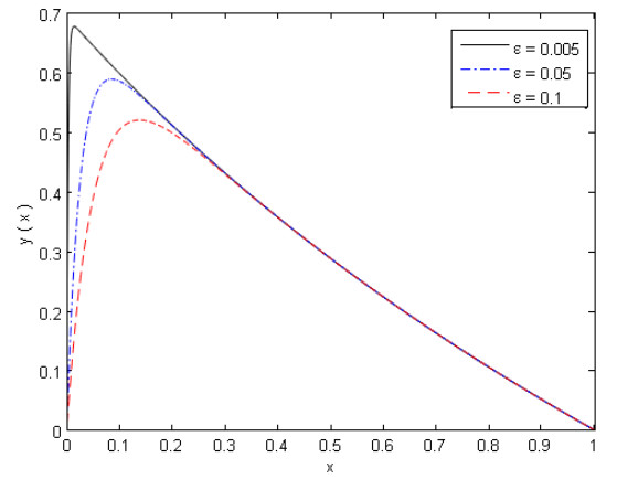
Example 1. Consider the nonlinear SPBVP from Bender and Orszag ^[6]

To solve this problem, we input the following command:

$spivp(2, exp(y), 0, 0)$

The output is:

which is the uniform valid approximate solution given by Bender and Orszag ^[6]. The solution of Example 1 at different values of $\varepsilon$ is presented in Figure 1.

Figure 1.  Solution of Example 1 at different values of $\varepsilon$.

DownLoad: Full-Size Img PowerPoint

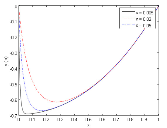
Example 2. Consider the nonlinear SPBVP from O'Malley ^[2]

Input the following command in Maple

$spivp(exp(y), -Pi/2.sin(Pi.x/2).exp(2.y), 0, 0)$;

The output is

which is the uniform valid approximate solution given by O'Malley ^[2]. The solution of Example 2 at different values of $\varepsilon$ is presented in Figure 2.

Figure 2.  Solution of Example 2 at different values of $\varepsilon$.

DownLoad: Full-Size Img PowerPoint

As shown from the previous two examples, the present algorithm offers a simple and easy tool for obtaining asymptotic analytical and approximate numerical solutions for SPBVPs.

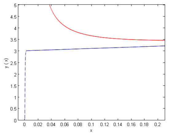
Example 3. Consider the nonlinear SPBVP from Kevorkian and Cole ^[7]

For comparison purpose, we write the uniform approximation provided by Kevorkian and Cole ^[7] as

where $c_{1} = 2.9995$ and $c_{2} = 1/c_{1}\ln[(c_{1}-1)/(c_{1}+1)]$.

For this problem, Wang ^[9] has obtained a solution given by:

where $t = x/\varepsilon$, and

where $\delta = -1.999791999$.

Here we apply the present method by inputting the following command in Maple

$spivp(y, - y, -1, 3.9995)$;

The output is

In Figure 3, the present solution (5.7) and the obtained solutions by Wang ^[9], Eqs. (5.5-5.6) are compared with the uniform approximate solution in ^[7] at $\varepsilon = 0.001$. As shown from Figure 3 the solution (5.5-5.6), solid red line, deviates much from our solution (5.7), dashed blue line, and the uniform approximate solution, dotted blue line, in ^[7]. In fact, applying the condition$\mathop{\lim }\limits_{t\to +\infty }v(t) = 0$ to (5.6) results in two different values for $\delta$ $(\delta = -1.999791999$, $\delta = -0.5$) and each one of them leads to unsatisfied results. The numerical results of Example 3 are compared with the results in literature in Table 1. Moreover, the results for different values of $\varepsilon$ are presented in Table 2.

Figure 3.  Comparison of the numerical solutions of Example 3 at $\varepsilon = 0.001$.

DownLoad: Full-Size Img PowerPoint

Table 1.  Comparison of the numerical solutions of Example 3 at $\varepsilon = 10^{-3}$.

x	Present	Results in[16]	Results in[17]	Results in[7]
0.00	-1.000000	-1.000000	-1.000000	-1.0000000
0.5$\varepsilon$	1.1484593	2.1363630	1.1484592	1.1484592
1.0$\varepsilon$	2.4569397	2.8140590	2.4569396	2.4569396
0.1	3.0994999	3.0995020	3.0962686	3.0994999
0.2	3.1995000	3.1995020	3.1963699	3.1995000
0.3	3.2995000	3.2995020	3.2964650	3.2995000
0.4	3.3995000	3.3995010	3.3965544	3.3995000
0.5	3.4995000	3.4995010	3.4466386	3.4995000
0.6	3.5995000	3.5995000	3.5967184	3.5995000
0.7	3.6995000	3.6995000	3.6967939	3.6995000
0.8	3.7995000	3.7995000	3.7968656	3.7995000
0.9	3.8995000	3.8995000	3.8969335	3.8995000
1.0	3.9995000	3.9995000	3.9969980	3.9995000

---

 | Show Table

DownLoad: CSV

Table 2.  Solution of Example 3 at different values of $\varepsilon$.

x	$\varepsilon=10^{-2}$	$\varepsilon=10^{-4}$	$\varepsilon=10^{-5}$	$\varepsilon=10^{-6}$
0.00	-1.0000000	-1.0000000	-1.0000000	-1.0000000
0.5$\varepsilon$	1.1529593	1.1480093	1.1479643	1.1479598
1.0$\varepsilon$	2.4659397	2.4560397	2.4559497	2.4559407
0.1	3.0995000	3.0995000	3.0995000	3.0995000
0.2	3.1995000	3.1995000	3.1995000	3.1995000
0.3	3.2995000	3.2995000	3.2995000	3.2995000
0.4	3.3995000	3.3995000	3.3995000	3.3995000
0.5	3.4995000	3.4995000	3.4995000	3.4995000
0.6	3.5995000	3.5995000	3.5995000	3.5995000
0.7	3.6995000	3.6995000	3.6995000	3.6995000
0.8	3.7995000	3.7995000	3.7995000	3.7995000
0.9	3.8995000	3.8995000	3.8995000	3.8995000
1.0	3.9995000	3.9995000	3.9995000	3.9995000

---

 | Show Table

DownLoad: CSV

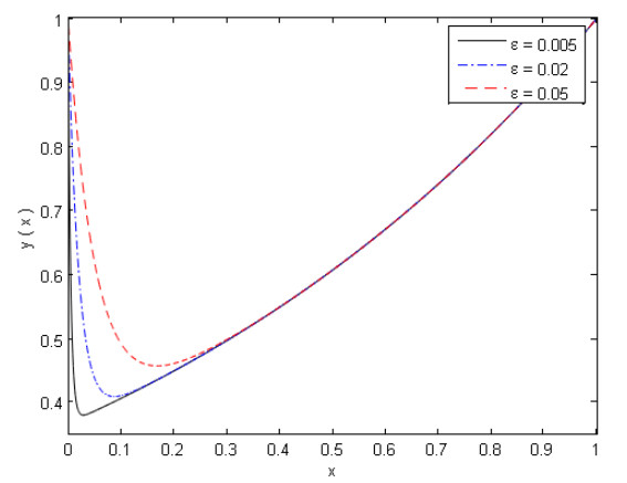
Example 4. Finally, we consider the following linear SPBVP from Bender and Orszag ^[6]

For this problem, Wang ^[9] has obtained the following rational solution:

where

and

Using the following command :

$spivp (1, -y, 1, 1)$,

the obtained solution is

The numerical results of Example 4 are shown in Tables 3, 4 and Figure 4.

Table 3.  Comparison of the numerical solutions of Example 4 at $\varepsilon = 10^{-3}$.

x	Present	Results in[6]	Results in[9]	Results in[17]	Exact solution
0.00	1.0000000	1.0000000	1.0000000	1.0000000	1.0000000
0.01	0.3716054	0.3716050	39.621608	0.3712379	0.3719724
0.02	0.3753111	0.3753109	34.943933	0.3749439	0.3756784
0.03	0.3790831	0.3790832	29.856212	0.3787160	0.3794502
0.04	0.3828929	0.3828929	25.706355	0.3825260	0.3832599
0.05	0.3867410	0.3867409	22.458425	0.3863742	0.3871079
0.10	0.4065697	0.4065696	13.632736	0.4062043	0.4069350
0.30	0.4965853	0.4965853	5.5064473	0.4962382	0.4969324
0.50	0.6065307	0.6065305	3.6923714	0.6062278	0.6068334
0.70	0.7408182	0.7408182	2.9700713	0.7405963	0.7410401
0.90	0.9048374	0.9048373	2.6496651	0.9047471	0.9049277
1.00	1.0000000	1.0000000	2.5738182	1.0000000	1.0000000

---

 | Show Table

DownLoad: CSV

Table 4.  Solution of Example 4 at different values of $\varepsilon$.

x	$\varepsilon=10^{-2}$	$\varepsilon=10^{-4}$	$\varepsilon=10^{-5}$	$\varepsilon=10^{-6}$
0.00	1.00000000	1.000000000	1.00000000	1.00000000
0.01	0.60412084	0.37157669	0.37157669	0.37157669
0.02	0.46085931	0.37531109	0.37531109	0.37531109
0.03	0.41055446	0.37908303	0.37908303	0.37908303
0.04	0.39447057	0.38289288	0.38289288	0.38289288
0.05	0.39100021	0.38674102	0.38674102	0.38674102
0.10	0.40659835	0.40656965	0.40656965	0.40656965
0.30	0.49658530	0.49658530	0.49658530	0.49658530
0.50	0.60653065	0.60653065	0.60653065	0.60653065
0.70	0.74081822	0.74081822	0.74081822	0.74081822
0.90	0.90483741	0.90483741	0.90483741	0.90483741
1.00	1.00000000	1.00000000	1.00000000	1.00000000

---

 | Show Table

DownLoad: CSV

Figure 4.  Solution of Example 4 at different values of $\varepsilon$.

DownLoad: Full-Size Img PowerPoint

Obviously, the solution in (5.9) needs more higher-order terms in Pade's expansion to match the boundary layer behavior ^[10].

6.   Conclusion

In this paper, we have presented approximate analytical and numerical solution of SPBVPs using a new and simple Maple program spivp. The method is based on an initial value method that replaces the original SPBVP by two asymptotically approximate IVPs. These IVPs are solved analytically and their solutions are combined to approximate the analytical solution of the original SPBVP. The method is very easy to implement on any computer with a minimum problem preparation. We have implemented it in Maple and applied it to four examples and compared the obtained results with the results in literature. The results indicate that the method is accurate and offers a simple and easy practical tool for the practicing engineers or applied mathematicians who need a practical tool for obtaining approximate analytical and numerical solution of SPBVPs.

Acknowledgment

The author would like to thank the referees for their valuable comments and suggestions which helped to improve the manuscript. Moreover, the author acknowledges that this publication was supported by the Deanship of Scientific Research at Prince Sattam bin Abdulaziz University, Saudi Arabia.

Conflict of interest

The author declares no conflict of interest.