Min | Mean | Median | SD | Max | |
Gbp | 1.149 | 1.533 | 1.534 | 0.222 | 2.108 |
Eur | 1.039 | 1.258 | 1.261 | 0.128 | 1.599 |
Jpy | 75.740 | 103.565 | 107.164 | 12.768 | 125.629 |
Aud | 0.574 | 0.829 | 0.783 | 0.120 | 1.103 |
Cny | 6.031 | 6.696 | 6.652 | 0.453 | 8.022 |
Citation: Bindusri Nair, B. Geetha Priyadarshini. Process, structure, property and applications of metallic glasses[J]. AIMS Materials Science, 2016, 3(3): 1022-1053. doi: 10.3934/matersci.2016.3.1022
[1] | Kai R. Wenger, Christian H. Leschinski, Philipp Sibbertsen . The memory of volatility. Quantitative Finance and Economics, 2018, 2(1): 622-644. doi: 10.3934/QFE.2018.1.137 |
[2] | Samuel Kwaku Agyei, Ahmed Bossman . Investor sentiment and the interdependence structure of GIIPS stock market returns: A multiscale approach. Quantitative Finance and Economics, 2023, 7(1): 87-116. doi: 10.3934/QFE.2023005 |
[3] | Lorna Katusiime . Time-Frequency connectedness between developing countries in the COVID-19 pandemic: The case of East Africa. Quantitative Finance and Economics, 2022, 6(4): 722-748. doi: 10.3934/QFE.2022032 |
[4] | Korhan Gokmenoglu, Baris Memduh Eren, Siamand Hesami . Exchange rates and stock markets in emerging economies: new evidence using the Quantile-on-Quantile approach. Quantitative Finance and Economics, 2021, 5(1): 94-110. doi: 10.3934/QFE.2021005 |
[5] | Elvira Caloiero, Massimo Guidolin . Volatility as an Alternative Asset Class: Does It Improve Portfolio Performance?. Quantitative Finance and Economics, 2017, 1(4): 334-362. doi: 10.3934/QFE.2017.4.334 |
[6] | Hongxuan Huang, Zhengjun Zhang . An intrinsic robust rank-one-approximation approach for currency portfolio optimization. Quantitative Finance and Economics, 2018, 2(1): 160-189. doi: 10.3934/QFE.2018.1.160 |
[7] | Kim Hiang Liow, Jeongseop Song, Xiaoxia Zhou . Volatility connectedness and market dependence across major financial markets in China economy. Quantitative Finance and Economics, 2021, 5(3): 397-420. doi: 10.3934/QFE.2021018 |
[8] | Mustafa Tevfik Kartal, Özer Depren, Serpil Kılıç Depren . The determinants of main stock exchange index changes in emerging countries: evidence from Turkey in COVID-19 pandemic age. Quantitative Finance and Economics, 2020, 4(4): 526-541. doi: 10.3934/QFE.2020025 |
[9] | Wenhui Li, Normaziah Mohd Nor, Hisham M, Feng Min . Volatility conditions and the weekend effect of long-short anomalies: Evidence from the US stock market. Quantitative Finance and Economics, 2023, 7(2): 337-355. doi: 10.3934/QFE.2023016 |
[10] | Lukáš Pichl, Taisei Kaizoji . Volatility Analysis of Bitcoin Price Time Series. Quantitative Finance and Economics, 2017, 1(4): 474-485. doi: 10.3934/QFE.2017.4.474 |
Foreign exchange (FOREX) is one of the main macroeconomic indicators for determining the stability of any economy and for country-country economic and financial status comparison. It generally measures the strength of a nation's local currency compared to currency of another country that is a trading partner. For global trade in the era of open economy with increasing competitiveness, FOREX has been one of the key factors (Kartono et al., 2020). Changes in exchange rates have a substantial impact on the economy and financial markets, e.g., since oil and global commodities are traded in US dollar, fluctuations in US dollar exchange rates lead to appreciation/depreciation of local currencies. To oil exporting countries, more US dollar reserve is accrued when local currencies appreciate against the US dollar, while to the oil importing countries, more US dollars are needed to keep up with the purchase of oil from the oil producers. Similarly, the depreciation of local currencies also has a large effect on the foreign reserve of a given nation. Thus, the present study is relevant among researchers and policymakers.
Prominent US dollar exchange rates are the US dollar rates to the British pound, euro, Japanese yen, Australian dollar and Chinese yuan. These exchange rates are highly traded and exhibit high volatility due to globalization according to Anjum and Msalik (2020). The authors further stated that trading partners are manipulating their exchange rates by using quantitative easing and managed exchange rates in order to increase price competitiveness for exporters, while countries that actively manage their currency rates, such as Japan and China, adhere to open markets and flexible exchange rates. As they experience an appreciation of their local currencies, they reduce dependence on imported goods and services.
Several papers have investigated the dynamic relationship between a group of prominent exchange rates with a focus on the US dollar rate for currencies such as the euro, British pound and Japanese yen as documented in Section 2. However, no research has yet connected the volatility's long-term memory property to the actual level of asset values and checked if cointegration and dynamic connectedness have a connection econometrically. From the survey of literature, only the work of Hung et al. (2022) considered datasets similar to ours. The authors analyzed the daily US dollar exchange rates to the euro, British pound, Canadian dollar, Australian dollar, the Swiss franc and Japanese yen between January 1st to May 12th, 2021. They analyzed a variant of multivariate volatility models to investigate the equicorrelation and association between currencies.
In this paper, we investigate cointegration and dynamic connectedness in market volatility of prominent exchange rates, focusing on US dollar exchange rates to the British pound, European euro, Japanese yen, Australian dollar and Chinese yuan. We employ an updated fractional cointegration framework that relies on cointegrating vector estimates from the narrow-band frequency domain least squares (NBFDLS) estimator in obtaining the residuals from the cointegrating variable pairs. The ordinary least squares (OLS) estimator is standard, but its estimates are usually biased. The NBFDLS estimator of Christensen and Nielsen (2006) is preferred to the OLS estimator and least square estimator in the frequency domain with periodograms as in Robinson (1994a). We also consider the quantile connectedness approach to investigate extreme up (bull) and down (bear) market fluctuations in the volatility of exchange rate by considering exchange rate pairs. Specifically, we employ the quantile vector autoregressive (QVAR) framework, recently proposed by Chatziantoniou et al. (2021) to investigate the dynamic connectedness over time, across three market conditions defined as normal market, the bear market and the bull market.1 Dynamic connectedness also indicates the transmission of volatility shocks by indicating if a variable is a transmitter or a receiver of shock as indicated in the net total connectedness. Furthermore, FOREX trading portfolio management strategies are applied (see Yaya et al., 2016; Furuoka et al., 2023; Wu et al., 2023). Since the fractional cointegration is related with a quantile dynamic connectedness methodology to uncover previously unknown features of monetary relationships in this paper, the unusual combination of methodologies presented here heralds a new path for greater understanding of the interdependence of global currencies and will serve as guide to regulators and portfolio managers.
1The Quantile VAR framework of Chatziantoniou et al. (2021) is an upgrade to the generalized VAR and spillover index of Diebold and Yilmaz (2012), and Diebold and Yılmaz (2014). It measures dynamic connectedness for various quantile values 0<τ<1.
The findings in the paper are quite interesting as we observe cointegration in some pairs of exchange rates, particularly those including the euro and British pound. Furthermore, the analyses of dynamic connectedness for the three market conditions (bear, normal and bull) indicate heterogeneity in net transmission of volatility, while cases of weak average connectedness are tallied with those cases of no cointegration. FOREX pairs including the British pound, or the euro showed stronger connectedness indices compared to others. The results of portfolio management strategies show similar results to these and could serve as a guide to FOREX traders and government decision-makers.
The rest of the paper is therefore structured as follows: Section 2 presents the review of some literature. Section 3 presents the time series econometric method used in the entire paper. Section 4 presents the data, empirical results and discussion. Section 5 concludes the paper.
The study of cointegration among exchange rates is a cornerstone in comprehending the global financial market's interconnectedness and long-term equilibrium relationships. This comprehensive review of literature takes readers on a voyage through the expanding terrain of techniques and empirical evidence, giving insight on the intricacies inherent in these interconnected currency dynamics. Arize (1995) studied the impact of real exchange-rate volatility on the trade flows of Denmark, the Netherlands, Sweden and Switzerland by applying a system-based cointegration of Johansen (1991), Johansen and Juselius (1990) and multivariate error-correction model. Their findings revealed that an increase in the volatility of the real exchange rate and approximating exchange-rate uncertainty exerts a significant negative effect on export demand in both the short-run and the long-run. Using a multivariate cointegration method of Johansen (1988) and Johansen and Juselius (1990) on monthly data of US dollar/German mark (DM) exchange rates that spanned 20 years, Kim and Mo (1995) revealed that the cointegration relationship among the series of I(1) can be represented by an error-correction model. They also showed that the random walk model outperformed the monetary structural models in the short run, while monetary structural models outperformed the random walk model in the long run according to the error-correction model.
Lin et al. (1998) used a generalized linear cointegration model on the daily spot exchange rates of the US dollar against the Japanese yen, the German mark, the Singapore dollar and the Swiss franc to identify complex long-run relationships in exchange rates that might not be detectable under simple linear cointegration models. Their findings revealed that complex linear forms of cointegration could exist even where current simple linear cointegration models reveal no evidence of cointegration. Martinez (1999) investigated whether a statistical long-run relationship is observed in Mexico's balance-of-payments and exchange rate. By using a cointegration technique and innovation accounting techniques, the authors found a long-run relationship between changes in international reserves and the exchange rate and changes in domestic credit. Mexico's monetary authorities adjusted domestic assets to sterilize balance-of-payments deficits in a futile attempt to control its monetary policy. Pan and Liu (1999) found that German mark, British pound, Japanese yen, Canadian dollar, French franc, Italian lira and Swiss franc vis-a-vis the U.S. dollar are cointegrated in the usual way for a 1985–1992 sample data. The suggestion is that if there's a fractional cointegration feature within exchange rates, it is possible that this feature is not constant and could vary across different time periods. The cointegrating relationship between DM–US dollar and the yen–US dollar real exchange rates possesses long memory in terms of monetary and real factors. Only a combination of real and monetary variables can accurately track down the movements of real exchange rates (Caporale and Gil-Alana, 2004). Kang (2008) examined the cointegration relationships of foreign exchange rates of Group of Seven (G-7) countries using the Ordinary Least Squares (OLS), Maximum Likelihood Estimator (MLE) and search methods. The findings revealed bivariate cointegrations and irreducible trivariate cointegration relationships among the G-7 countries exchange rates. The search method is shown to be an effective method to find cointegration relationships. Gil-Alana and Carcel (2020) examined the cointegrating structure of British pound, the Euro, the Swedish Krona, the Canadian dollar and the Swiss Franc to the US dollar using fractional integration and fractionally cointegrated VAR by Johansen and Nielsen (2012). The findings revealed that the five exchange rates are not cointegrated in a classical way, and although they possessed long memory, the exchange rate dynamic is fractionally cointegrated.
Alessandro (2019) investigated cointegration relationships across the exchange rates of the international currencies (IC) using the Johansen cointegration test, the standard test for unit root and the augmented Dickey-Fuller test for USD/euro, and they suggested the series had a unit root in the process because the information criteria for the series considered one lag. Using volatility spillover index and LASSO-VAR approaches to examine the total and directional volatility connectedness in global foreign exchange (forex) markets, Wen and Wang (2020) found that total volatility connectedness reacts sensitively to changes in international economic fundamentals and increases during crisis periods. The authors found that oil exports, forex regimes and monetary policies are major factors driving volatility transmission across global forex markets.
Huynh et al. (2020) examined the directional spillover effects and connectedness for return and volatility of nine US dollar exchange rates of the most globally traded currencies under the influence of trade policy uncertainty. Using generalized VAR and the spillover index of Diebold and Yilmaz (2012) and Diebold and Yılmaz (2014), their findings revealed asymmetric spillovers and connectedness among the considered exchange rates when trade policy uncertainty is present and volatility spillover is stronger than the return connectedness between exchange rate and trade policy uncertainty. Gabauer (2021) used a time-varying parameter vector autoregressive framework (TVP-VAR) with a time-varying variance-covariance structure on daily exchange rate data of 15 countries to the US dollar to investigate whether countries in a currency area face symmetric shock or not. The findings revealed that the net transmitters are Austria, Belgium, Denmark, Germany, Luxembourg, France, the Netherlands, Ireland and Italy. They also revealed the existence of a small and stable optimum currency area (OCA) among Austria, Germany and the Netherlands and an extended less stable OCA, including the first OCA members and Belgium, Denmark, France and Luxembourg. Hung et al. (2022) examined the equicorrelation and causal association across major currency markets during the COVID-19 pandemic. Adopting the DECO-GARCH model developed by Engle and Kelly (2012), the transfer entropy approach and using the daily data of exchange rates of the US dollar to euro (EURO), the Canadian dollar (CAN), the British pound (GBP), the Australian dollar (AUD), the Swiss franc (CHF) and the Japanese yen (YEN), the findings revealed a bidirectional relationship between exchange rate returns. The COVID-19 outbreak triggers the spillover effects between significant exchange rates returns.
The methodology applied in the present paper is novel and has not been previously applied in all the literature listed above. Long memory cointegration test based on NBFDLS estimator is recently applied in Yaya et al. (2023) to climatological datasets, while this present paper considers long memory cointegration and quantile dynamic connectedness to investigate possible linkages.
The standard non-seasonal I(d) is given as follows:
(1−L)dxt=ut,t=1,2,..., | (1) |
where d is any real number in fractional and integer values. The lag operator is L, defined such that Lxt = xt-1, while ut represents the I(0) white noise process. The left side of the difference operator in (1) is expanded using the binomial expression. Thus,
(1−L)d=∞∑j=0(dj)(−1)jLj=1−dL+d(d−1)2L2−… |
such that
(1−L)dxt=xt−dxt−1+d(d−1)2xt−2−… |
and
xt=dxt−1+d(d−1)2xt−2+⋯+ut. | (2) |
The expansion in (2) is used for fractional differencing with a certain d value. The expression shows the dependence/correlation between xtand its lagged values xt−i, where i is a certain time in the past.
The fractional dependence parameter d has been estimated by many methods, among which are semi-parametric and parametric methods. In the frequency domain, the semi-parametric local Whittle estimation method by Robinson (1995) is a common semiparametric technique. The parametric technique uses the parametric frequency domain Whittle estimation approach (Dahlhaus, 1989), with a testing procedure of Robinson (1994b), which is a Lagrange multiplier (LM) principle, using the null hypothesis,
H0:d=d0, | (3) |
provided d0 are real values. Robinson (1994b) extended (1) using the linear deterministic function as in the augmented Dickey-Fuller (ADF) regression. Thus, (1) becomes (4) below,
yt=β0+β1t+xt,(1−L)dxt=ut,t=1,2,… | (4) |
where β0 and β1 are the intercept and slope parameters, respectively, for trend t in the model. The significance of β1 in the entire estimation process informs the relevance/preference of the deterministic term over others. By respecifying the two equations in (4) as a single one, we have
y∗t=β01∗t+β1t∗t+ut,t=1,2,…, | (5) |
where y∗t=(1−L)doyt; 1∗t=(1−L)do1t; t∗t=(1−L)dott. With the fact that ut is still an I(0) process by construction, we can then estimate β0 and β1 in (5) by standard OLS methods, such that the estimated residuals are
ˆut=y∗t−ˆβ01∗t+ˆβ1t∗t,t=1,2,…, | (6) |
For robustness, the results of fractional integration obtained using the parametric approach of Robinson (1994b) are supported with those obtained using the semiparametric method of Robinson (1995). The attractiveness of the semi-parametric methods is that no validation of assumption on the error term is required. The local Whittle (LW) estimator in the frequency domain is employed, and this uses a frequency band that degenerates to zero. This method is proposed by Robinson (1995), and it uses the estimator,
ˆd=argmind(logC∗(d)−2d1m∑mj=1logλj), | (7) |
where d∈(−12,12)and
¯C(d)=1m∑mj=1I(λj)λ2dj;λj=2πjT,1m+1T→0,
where m stands for the parameter of bandwidth, while I(λj) is the periodogram of the time series, xt specified as
I(λj)=12πT|n∑t=1xteiλjt|2. |
Robinson (1995) showed that under the finiteness of the fourth moment and other very mild conditions,
√m(ˆd−d0)d→N(0,14)asT⟶∞, |
with the actual value of d, represented by d0.
The homogeneity test of paired integration orders by Robinson and Yajima (2002) is necessary in the case of fractional differencing, while Engle and Granger (1987) have relaxed the unit differencing condition to be of any real number. This makes the extension to fractional cointegration easier. Thus, equality of fractional order needs to be established by testing for non-significance differences in the distribution of the differencing order based on the null,
H0:dy1=dy2, | (8) |
where dy1 and dy2 are the two integration orders from the paired series (y1t,y2t). The test statistic is given as
ˆTxy=m1/2(ˆdy1−ˆdy2){12[1−ˆG2y1,y2/(ˆG2y1ˆG2y1,y2)]}1/2+h(T), | (9) |
where h(T)>0 and ˆG2y1,y2 represents the (y1×y2)th element of ˆΛ(λj)−1I(λj)ˆΛ(λj) with ˆΛ(λj)=diag{eiπˆdy1/2λ−ˆdy1,eiπˆdy2/2λ−ˆdy2}. The test is normally distributed with a two-sided critical value of approximately 1.96. Thus, once equality of fractional integration orders is reached, a fractional cointegration test is carried out; this is described in the next sub-section.
The narrow band frequency domain least square (NBFDLS) must estimate be considered to obtain the cointegrating vector linking the paired variables provided that the variables possess long memory properties with weakly dependent regressors. Thus, the regressors and the residuals are correlated, even over a long-time span. The NBFDLS is a semi-parametric estimator that applies the OLS on a degenerated band of frequencies around the origin, as proposed in Robinson (1994a), with further modification and current software implementation in Christensen and Nielsen (2006) for stationary time series.
In the two-variable case, i.e., y1t and y2t for fractional integration orders (0<d<0.5) and residuals of order de<d, the NBFDLS estimator can be written as
ˆβ={1m∑mj=1Re[Iy1,y1(λj)]}−1x1m∑mj=1Re[Iy1,y1(λj)] | (10) |
which as m approaches infinity, tends to be distributed as,
√mλde−dm(ˆβ−β0)d→N[0,ge(1−2d)22gy1(1−2d−2de)] | (11) |
where gy1 and ge are the 2×2G diagonal matrix elements. It can be seen from (10), that as long as d+de<0.5, normality is always ensured (see Christensen and Nielsen, 2006).
The strength and transmission of volatility shocks between the two return variables y1t and y2t being investigated is known as the connectedness analysis. The quantile vector autoregressive (QVAR) dynamic connectedness method was proposed by Chatziantoniou et al. (2021). In light of this, the connectedness between the paired exchange rates for the 5th (lower) quantile, 50th (median) quantile and 95th (upper) quantile are investigated. The approach uses the estimate of the quantile VAR(p) model defined using quantile, τ:
Xt=μ(τ)+∑pj=1Φj(τ)Xt−j+ut(τ), | (12) |
where the Xt is the vector of 2×1 dimensional endogenous variables Xt = (y1t, y2t) and τ is the quantile with values ranging between 0 and 1 towards the 5th quantile and 95th quantile, respectively. The 50th quantile (τ = 0.50) explains the normal market condition, and the bearish and bullish market conditions are found at the lower (τ=0.05) and upper (τ=0.95), respectively. Then, p gives the order of the quantile VAR model as shown in (12). The conditional mean vector of 2×1 is represented by μ(τ), the 2×2 dimensional autoregressive model coefficient matrix is denoted by Φj(τ), the 2×1 dimensional error vector with a 2×2 dimensional variance-covariance matrix ∑(τ),denoted by ut(τ). Using the world's representation, the QVAR(p) is converted to a quantile vector moving average [QVMA(∞)} thus:
Xt=μ(τ)+∑∞i=0Ψi(τ)ut−i | (13) |
where Ψi is the 2×2 dimensional matrix of moving average coefficients and ut−i are the moving average innovations. This is approach is suggested by Koop et al. (1996) and Pesaran and Shin (1998) and is necessary for determining the connectedness between any two markets in terms of returns and variance. It is the H-step ahead generalized forecast error variance decomposition (GFEVD) given as,
Ψτij(H)=∑(τ)−1ii∑H−1h=0(e'iΨh(τ)∑(τ)ej)2∑H−1h=0(e'iΨh(τ)∑(τ)Ψh(τ)'ei | (14) |
which transforms to
˜Ψτij(H)=Ψτij(H)∑kj=1Ψτij(H), | (15) |
where ei in (14) represents a zero vector which equals unity on the ith position, which also results in two equalities in (15), i.e., ∑kj=1˜Ψτij(H)=1 and ∑ki,j=1˜Ψτij(H)=k. The influence of variable j on another variable i in terms of its share of forecast error variance/shocks is being measured by ˜Ψτij(H), and this is defined as the total directional connectedness to others, that is, Cgi←j(H), which is the directional volatility spillovers from j to i. Also, the influence received by variable j from another variable i, which is the total directional connectedness FROM others is computed as Cgi→j(H) which is the directional volatility spillover from i to j. The net directional connectedness is then calculated as
NETτ=Cτi←j(H)−Cτi→j(H) | (16) |
If NETτ is greater than 0, it means variance shock in that variable influences the second variable more than it is being influenced, but if NETτ is less than 0, this implies that the variable is being dominated by the other variable in terms of variance shock. Thus, in cases where NETτ>0, the variable is a net transmitter of shocks, while in cases where NETτ<0, the variable is a net receiver of shock. The total connectedness index (TCI) between variables i and j is given in (16) and can be expressed as:
TCIτ=∑ki,j=1,i≠j˜Ψτij(H)k−1, | (17) |
where this gives the strength of the connectedness in the paired variables. If the TCI is high, it means high market risk between the two assets and they influence each other more strongly, but if it is low, it means low market risk, as the two assets influence each other weakly.
Daily US dollar exchange rates to the Australian dollar (AUD), Chinese yuan (CNY), European euro (EUR), British pound (GBP) and Japanese yen (JPY) were used in this study. The data spanned May 16, 2006, to August 10, 2022, and were retrieved from the Yahoo Finance website (https://www.finance.yahoo.com). The descriptive statistics are presented in Table 1. We observed a noticeable variation in the exchange rate of the Japanese yen. Other exchange rates appear to be distributed normally, having approximately equal mean and median values. Plots of these exchange rates are given in Figure 1, along with each corresponding log-returns since the focus is on volatility, which is visible with the log-returns plot. For USD/AUD, USD/EUR, USD/GBP and USD/JPY, we observe a general decreasing trend over the historical years. This implies that the local currencies, the Australian dollar, euro, British pound, and Japanese yen have appreciated against the US dollar over the years. The only exception is USD/CNY, in which the Chinese yuan has depreciated against the US dollar over the years. A closer look at the log-returns plot indicates possible higher volatility in the case of USD/AUD, USD/CNY and USD/GBP exchange rates, which explains that those FOREX markets are more turbulent than the remaining markets (USD/EUR and USD/JPY).
Min | Mean | Median | SD | Max | |
Gbp | 1.149 | 1.533 | 1.534 | 0.222 | 2.108 |
Eur | 1.039 | 1.258 | 1.261 | 0.128 | 1.599 |
Jpy | 75.740 | 103.565 | 107.164 | 12.768 | 125.629 |
Aud | 0.574 | 0.829 | 0.783 | 0.120 | 1.103 |
Cny | 6.031 | 6.696 | 6.652 | 0.453 | 8.022 |
Table 2 presents the results of volatility persistence in the three FOREX markets. The log returns have been transformed into absolute returns used as a proxy for volatility here. Estimates of fractional integration are obtained from the absolute return series, based on Robinson's (1994b) framework. The selected model results are in bold for each exchange rate series. It is observed that USD/EUR and USD/JPY exchange rates present higher volatility persistence compared to USD/GBP, USD/AUD and USD/CNY, even though all these persistence are around 0.2. By linking these results with the observation in Figure 1, it means that USD/AUD, USD/CNY and USD/GBP exchange rates with higher volatility will persist less as the results revealed in Table 2. In addition, these volatilities are in a long memory range and external shocks targeted to them will be transitory.
Series | No terms | Intercept only | Intercept with time trend |
GBP | 0.153 (0.134, 0.172) | 0.153 (0.134, 0.172) | 0.152 (0.133, 0.171) |
EUR | 0.243 (0.218, 0.268) | 0.243 (0.218, 0.268) | 0.240 (0.215, 0.265) |
JPY | 0.238 (0.214, 0.262) | 0.238 (0.214, 0.262) | 0.234 (0.209, 0.259) |
AUD | 0.201 (0.182, 0.220) | 0.201 (0.182, 0.220) | 0.198 (0.179, 0.217) |
CNY | 0.186 (0.142, 0.230) | 0.186 (0.142, 0.230) | 0.182 (0.138, 0.226) |
Note: in bold are selected results obtained based on the significance of parameters of the deterministic terms in Robinson's (1994) framework. |
Next, in Table 3, we conducted homogeneity of fractional integration orders for the pairs following from the results of Robinson (1994b) in Table 2. Since we have included five US dollar exchange rate variables, these lead to 10 variable pairs as reported in Table 3.2 The t-statistics for the homogeneity test of Robinson and Yajima (2002) are reported in the table where no rejection of null hypotheses of equality of fractional orders for any pair of variables is observed.
Pairs | m = T0.5 | m = T0.6 |
GBP – EUR | 1.610 | 0.003 |
GBP – JPY | 0.757 | 0.073 |
GBP – AUD | 0.289 | 1.677 |
GBP – CNY | 0.005 | 0.196 |
EUR – JPY | 0.998 | 0.090 |
EUR – AUD | 1.355 | 1.640 |
EUR – CNY | 1.596 | 0.191 |
JPY – AUD | 0.499 | 1.722 |
JPY – CNY | 0.749 | 0.267 |
AUD – CNY | 0.265 | 1.382 |
Note: The homogeneity of fractional d is distributed normally, therefore the two-sided critical point is 1.96 at a 5% level. |
2Note, GBP is the USD/GBP exchange rate, EUR is the USD/EUR exchange rate and similarly to the remaining eight exchange rates.
Since our interest is on the behaviour of volatility pairs of the exchange rate, and with the notion of volatility series (absolute returns or square returns of asset prices) portraying long memory properties in which 0<d<0.5, we relied on an updated fractional cointegration beta estimator. The NBFDLS estimator is robust to testing fractional cointegration within the long memory range. The estimator uses bandwidth numbers mto obtain the residuals from the cointegrating vector of the variable pairs. This estimator relied on its β values for obtaining the residuals e as e=y2t−βy1t, where the paired series are (y1t,y2t). These β values are reported in Table 4 for the bandwidths m=T0.5 and T0.6. Estimates of residuals for cointegration obtained in this way using the NBFDLS estimator of Christensen and Nielsen (2006) are preferred to the standard OLS residuals for cointegration (see Yaya et al., 2023).
Pairs | m = T0.5 | m = T0.6 |
GBP – EUR | 0.492 | 0.415 |
GBP – JPY | 0.468 | 0.368 |
GBP – AUD | 0.423 | 0.418 |
GBP – CNY | 0.153 | 0.189 |
EUR – JPY | 0.720 | 0.703 |
EUR – AUD | 0.622 | 0.598 |
EUR – CNY | −0.401 | −0.212 |
JPY – AUD | 0.567 | 0.553 |
JPY – CNY | −0.309 | −0.187 |
AUD – CNY | −0.512 | −0.321 |
Then, the residual series e was estimated for fractional cointegration using Marinucci and Robinson (2001). The residual-based cointegration test uses the residuals e from the NBFDLS β values. For the cointegration of any pair, it was expected that the fractional difference value for a residual series, de<min(dy1,dy2) where dy1 and dy2 are the two integration orders from the paired series (y1t,y2t). In Table 5, we found no case of anti-persistence (−0.5<d<0) but all estimates of fractional orders for residuals are in the long memory range, with an upper bound limit of estimates quite below 0.3 in the two frequency bandwidths.
Pairs | m = T0.5 | m = T0.6 |
GBP – EUR | 0.141 (0.118, 0.163) | 0.137 (0.114, 0.159) |
GBP – JPY | 0.129 (0.107, 0.150) | 0.127 (0.105, 0.149) |
GBP – AUD | 0.087 (0.066, 0.108) | 0.087 (0.067, 0.108) |
GBP – CNY | 0.152 (0.133, 0.171) | 0.152 (0.133, 0.171) |
EUR – JPY | 0.144 (0.123, 0.166) | 0.146 (0.124, 0.168) |
EUR – AUD | 0.181 (0.153, 0.208) | 0.184 (0.156, 0.211) |
EUR – CNY | 0.243 (0.218, 0.268) | 0.243 (0.218, 0.268) |
JPY – AUD | 0.178 (0.152, 0.203) | 0.179 (0.154, 0.205) |
JPY – CNY | 0.238 (0.214, 0.262) | 0.238 (0.214, 0.262) |
AUD – CNY | 0.201 (0.182, 0.220) | 0.201 (0.182, 0.220) |
Table 6 summarized the results in Table 2 and Table 5, where the results in Table 2 have been paired and reported in the second column y1t- y2t of Table 6 and the cases where the fractional cointegration condition de<min(dy1,dy2) are satisfied as indicated. The results showed seven pairs indicating fractional cointegration: GBP – EUR, GBP – JPY, GBP – AUD, GBP – CNY, EUR – JPY, EUR – AUD and JPY – AUD.
Pairs | y1t - y2t | Residual-based fractional cointegration test | |
m = T0.5 | m = T0.6 | ||
GBP – EUR | 0.153 - 0.243 | 0.141* | 0.137* |
GBP – JPY | 0.153 - 0.238 | 0.129* | 0.127* |
GBP – AUD | 0.153 - 0.198 | 0.087* | 0.087* |
GBP – CNY | 0.153 - 0.186 | 0.152* | 0.152* |
EUR – JPY | 0.243 - 0.238 | 0.144* | 0.146* |
EUR – AUD | 0.243 - 0.198 | 0.181* | 0.184* |
EUR – CNY | 0.243 - 0.186 | 0.243 | 0.243 |
JPY – AUD | 0.238 - 0.198 | 0.178* | 0.179* |
JPY – CNY | 0.238 - 0.186 | 0.238 | 0.238 |
AUD – CNY | 0.198 - 0.186 | 0.201 | 0.201 |
Note: in bold and * indicates cases of de<min(dy1,dy2). |
The next research question is how strong are these comovements? Which exchange rate dominates the other in terms of volatility? The results of quantile dynamic connectedness are presented for the middle quantile (Table 7), lower quantile (Table 8), and upper quantile (Table 9). In the case of the middle quantile (normal market condition) in Table 7, the average total connectedness indices (TCIs) are generally low with the highest in this table being 27.88 in the case of the GBP – EUR pair. This agrees with the notion emanating from the cointegration results that USD/GBP and USD/EUR drive other exchange rates. The least in terms of connectedness is JPY – CNY pair with 6.00 TCI–this pair is not indicating cointegration–and the pair AUD – CNY with 6.20 TCI. At this middle quantile, GBP is a net transmitter of a shock to EUR, JPY and CNY markets, while EUR is a net transmitter of a shock to JPY and CNY markets. These results are generally heterogenous, possibly due to low TCIs observed during this market phase.
Pairs | NET | TCIτ | |
y1t | y2t | ||
GBP – EUR | Transmitter | Receiver | 27.88 |
GBP – JPY | Transmitter | Receiver | 12.71 |
GBP – AUD | Receiver | Transmitter | 24.59 |
GBP – CNY | Transmitter | Receiver | 6.20 |
EUR – JPY | Transmitter | Receiver | 22.13 |
EUR – AUD | Receiver | Transmitter | 25.61 |
EUR – CNY | Transmitter | Receiver | 7.61 |
JPY – AUD | Transmitter | Receiver | 15.77 |
JPY – CNY | Transmitter | Receiver | 6.00 |
AUD – CNY | Transmitter | Receiver | 6.20 |
Pairs | NET | TCIτ | |
y1t | y2t | ||
GBP – EUR | Receiver | Transmitter | 63.72 |
GBP – JPY | Undecided | Undecided | 53.69 |
GBP – AUD | Transmitter | Receiver | 64.00 |
GBP – CNY | Receiver | Transmitter | 39.55 |
EUR – JPY | Transmitter | Receiver | 60.01 |
EUR – AUD | Transmitter | Receiver | 63.28 |
EUR – CNY | Receiver | Transmitter | 39.69 |
JPY – AUD | Receiver | Transmitter | 56.81 |
JPY – CNY | Receiver | Transmitter | 38.33 |
AUD – CNY | Receiver | Transmitter | 41.79 |
Pairs | NET | TCIτ | |
y1t | y2t | ||
GBP – EUR | Transmitter | Receiver | 84.64 |
GBP – JPY | Receiver | Transmitter | 82.36 |
GBP – AUD | Receiver | Transmitter | 85.63 |
GBP – CNY | Receiver | Transmitter | 80.09 |
EUR – JPY | Transmitter | Receiver | 83.13 |
EUR – AUD | Receiver | Transmitter | 85.74 |
EUR – CNY | Receiver | Transmitter | 80.71 |
JPY – AUD | Transmitter | Receiver | 83.15 |
JPY – CNY | Receiver | Transmitter | 80.28 |
AUD – CNY | Receiver | Transmitter | 81.41 |
In Table 8, At the lower quantile, which is the bear market state, the average connectedness index (TCI) is higher compared to that of the normal market state. Thus, exchange rates are more strongly bounded in pairs. The GBP – EUR pair has a TCI of 63.72, GBP – AUD has a TCI of 64.00, EUR – JPY has a TCI of 60.01, EUR – AUD has a TCI of 63.28, while GBP – JPY pair has a TCI of 53.69, GBP – CNY has a TCI of 39.55 and EUR – CNY has a TCI of 39.69. Thus, the US dollar/British pound and the US dollar/euro form pairs with those US dollar exchange rates with TCI above 60. Also, in the bear market, the performance of the US dollar/British pound (GBP) and US dollar/euro are heterogeneous in terms of volatility spillovers.
At the bull market state (see Table 9), the average TCI increased, with at least 80.0 in each pair and the highest TCI was 85.63 for the GBP – AUD pair. Generally, the pairs involving GBP and EUR still present higher TCIs compared to pairs of other exchange rates not involving GBP and EUR. By relating these results of average TCI with that of cointegration, one can say that there is a connection between long-memory cointegration and dynamic connectedness. In terms of transmission of volatility, heterogeneity is also observed at the bull FOREX market phase. It is only in GBP – CNY pair that we observed homogeneity in the net transmission of volatility that the normal market, bear and bull market phases, where the US dollar/British pound (GBP) is consistently the net transmitter of volatility shock and US dollar/Chinese yuan (CNY) is consistently the net shock receiver.
It follows to investigate portfolio strategies necessary to be adopted by portfolio managers to maintain or maximize profits by minimizing risks encountered on daily basis. Antonakakis et al. (2020) have suggested using estimates of time-varying variance-covariances and time-varying conditional correlations from the DCC-GARCH-t-Copula model to obtain the dynamic portfolio weights of Kroner and Ng (1998) and hedge ratios of Kroner and Sultan (1993). Kroner and Ng (1998) suggested the measure,
wijt=hiit−hijthjjt−2hijt+hiit | (18) |
with wijt={0,wijt,1,if wijt<0 if 0⩽wijt⩽1if wijt>1, where wijt is the weight of FOREX i in a $1 portfolio of the two FOREX (i,j) at time t, which leaves the proportional weight of FOREX j in the same portfolio as wjit=(1−wijt), hjjt and hiit denote the conditional variance series from the volatility model of each asset and hijt is the corresponding covariance series at a time, t. In the case of USD-GBP and USD-CNY exchange rate pairs, the weight of USD-GBP FOREX in the $1 priced portfolio of the two assets is wgbp,cny,t, which leaves the corresponding weight of USD-CNY FOREX at 1−wgbp,cny,t. Another portfolio management strategy by Kroner and Sultan (1993) on risk-minimizing hedge ratio is given as,
βijt=hijthjjt | (19) |
where a low hedge ratio βijt between the two FOREX assets (i,j) suggests that the risk in FOREX i can be hedged by taking a short position in FOREX j markets. Similar to optimal portfolio weight in the case of the USD-GBP and USD-CNY pair above, the hedge ratio measure βgbp,cny,t implies that the risk at the USD-GBP exchange rate market can be hedged by taking a short position in the USD-CNY exchange rate market.
In Table 10, the results of average optimal weights (wijt) and hedge ratios (βijt) obtained are presented in the second column and the third column of the table, respectively. By looking at the optimal weights in a $1 portfolio worth of FOREX containing the British pound (GBP) and Australian dollar (AUD), about 73 cents of the British pound should be invested, which corresponds to about 27 cents of the Australian dollar. In portfolio pairs containing Chinese yuan with other currencies such as the Australian dollar, euro, British pound, and Japanese yen, it is observed that more than 90 cents of Chinese yuan are required to be invested as against about 10 cents remaining for the other paired currency in the portfolio to maintain the accrued profits over time. These are portfolio pairs with weaker dynamic connectedness reported earlier in this paper. Thus, FOREX portfolio weighting relates to dynamic connectedness.
Pairs | wijt | βijt |
GBP - AUD | 0.73 | 0.42 |
GBP - CNY | 0.07 | 0.40 |
GBP - EUR | 0.53 | 0.58 |
GBP – JPY | 0.54 | 0.14 |
EUR - AUD | 0.70 | 0.42 |
EUR - CNY | 0.09 | 0.60 |
EUR – GBP | 0.47 | 0.61 |
EUR – JPY | 0.53 | 0.21 |
AUD - CNY | 0.04 | 0.73 |
AUD - EUR | 0.30 | 0.64 |
AUD- GBP | 0.27 | 0.69 |
AUD – JPY | 0.42 | 0.10 |
CNY - AUD | 0.96 | 0.07 |
CNY - EUR | 0.91 | 0.08 |
CNY - GBP | 0.93 | 0.06 |
CNY – JPY | 0.89 | 0.03 |
JPY – AUD | 0.58 | 0.08 |
JPY - CNY | 0.11 | 0.16 |
JPY – EUR | 0.47 | 0.23 |
JPY – GBP | 0.46 | 0.14 |
Results of the hedge ratio in the last column of Table 10 are striking also as we observe that those portfolio pairs containing Chinese yuan with other currencies such as the Australian dollar, euro, British pound, and Japanese yen require 3–7% of the other currencies in pairs with Chinese yuan to shorten $1 long of those FOREX traded with the Chinese yuan.
In this study, we focus on US dollar exchange rates to the British pound, European euro, Japanese yen, Australian dollar, and Chinese yuan to simultaneously investigate cointegration and dynamic connectedness in markets volatility of prominent currency rate pairs. We employed an updated fractional cointegrating framework, that is the narrow-band frequency domain least squares estimator of Christensen and Nielsen (2006) for obtaining residual series from cointegrating vector pairs. This estimator is preferred to the classical least square estimator and the least square in the frequency domain with periodograms, as in Robinson (1994a), because it allows fractional cointegration in long memory range. Quantile connectedness technique was used to examine the volatility of exchange rate pairs for extreme bull and bear market movements and at the normal market condition. Thus, investigating both cointegration and dynamic connectedness in a unified framework in this paper is an attractiveness, even the quantile analyses which make the presentation extremely different from Hung et al. (2022).
We first found that seven paired cases, i.e., GBP-EUR, GBP-JPY, GBP-AUD, GBP-CNY, EUR-JPY, EUR-AUD and JPY-AUD, satisfied the fractional cointegration criterion based on the narrow-band frequency domain least squares estimator for cointegrating betas. Quantile connectedness results showed that the pairs that indicated cointegration coincided with cases of stronger connectedness at the normal market, bear, and the bull market condition. One can infer that the long-memory cointegration and dynamic connectedness are related based on the findings. Furthermore, during the three market conditions analyzed by quantiles, the transmission or receipt of volatility shocks is unaffected by market situations. The outcomes of the developed portfolio management strategies likewise agree with those of cointegration and quantile connectedness.
This work is therefore seen as a fresh extension to Hung et al. (2022) because our findings agree with those of the authors in the paper. Our findings will interest FOREX traders, government, and policymakers. This work is opened to scrutiny, and it can also be extended to other low-volume traded US dollar exchange rates using daily and tick-by-tick datasets.
The authors affirm that no artificial intelligence (AI) tools are used in the creation of this work.
The authors thank the editor and the three anonymous reviewers for their valuable suggestions that led to the success of this research work.
The authors have received no funding from any source in the preparation of this work.
The author declares no conflicts of interest in this paper.
[1] | Klement WJ, Willens RH, Dumez P (1960) Non-crystalline Structure in Solidified Gold-Silicon alloys. Nature 187: 869–870. |
[2] |
Tsai PH, Li JB, Chang YZ (2014) Fatigue properties improvement of high-strength aluminum alloy by using a ZrCu-based metallic glass thin film coating. Thin Solid Films 561: 28–32. doi: 10.1016/j.tsf.2013.06.085
![]() |
[3] | Chu JP, Huang JC, Jang JSC (2010) Thin film metallic glasses: Preparations, Properties and Applications. J Miner Met Mater Soc 62: 419–424. |
[4] | Schroers J, Kumar G, Thomas M (2009) Bulk metallic glasses for biomedical applications. Bio Mater Dev 61: 21–29. |
[5] | Subir S (1992) Icosahedral ordering in supercooled liquids and metallic glasses. Bond Orientational order in Condensed Matter System. KJ Strandburg ed., Springer-Verlag, New York, 255–283. |
[6] |
Inoue A (2000) Stabilization of metallic supercooled liquid and bulk amorphous alloys. Acta Mater 48: 279–306. doi: 10.1016/S1359-6454(99)00300-6
![]() |
[7] | Inoue A (2001) Bullk amorphous and nanocrystalline alloys with high functional properties. Mater Sci Eng A 304: 1–10. |
[8] |
Turnbull D (1969) Under what conditions can a glass be formed. Contemp Phys 10: 473–488. doi: 10.1080/00107516908204405
![]() |
[9] |
Chu JP, Lee CM, Huang RT (2011) Zr-based glass-forming film for fatigue-property improvements of 316L stainless steel annealing effects. Surf Coat Tech 205: 4030–4034. doi: 10.1016/j.surfcoat.2011.02.040
![]() |
[10] |
Sun YT, Cao CR, Huang KQ (2014) Understanding glass-forming ability through sluggish crystallization of atomically thin metallic glassy films. Appl Phys Lett 105: 051901-051901-4. doi: 10.1063/1.4892448
![]() |
[11] | Ramakrishna BR (2009) Bulk metallic glasses: Materials of future. DRDO Sci Spectrum. |
[12] |
Inoue A, Zhang W (2004). Formation, thermal stability and mechanical properties of Cu-Zr and Cu-Hf binary glassy alloy rods. Mater Trans 45: 584–587. doi: 10.2320/matertrans.45.584
![]() |
[13] |
Kwon OJ, Kim YC, Kim KB (2006) Formation of amorphous phase in the binary Cu-Zr alloy system. Met Mater Int 12: 207–212. doi: 10.1007/BF03027532
![]() |
[14] | Samwer K, Johnson WL (1983) Structure of glassy early-transition-metal-late-transition-metal hydrides. Phys Rev B 28: 2907–2913. |
[15] |
Schwarz RB, Johnson WL (1983) Formation of an amorphous alloy by solid state reaction of the pure polycrystalline metals. Phys Rev Lett 51: 415–418. doi: 10.1103/PhysRevLett.51.415
![]() |
[16] | Linker G (1986) Strain induced amorphization of niobium by boron implantation. Solid State Commun 57: 773–776. |
[17] |
Sziraki L, Kuzmann E, El-SharifM (2000) Electrochemical behavior of electrodeposited strongly disordered Fe-Ni-Cr alloys. Electrochem Commun 2: 619–625. doi: 10.1016/S1388-2481(00)00088-6
![]() |
[18] |
Schwarz RB, Petrich RR, Saw CK (1985) The synthesis of amorphous NiTi alloy powders by mechanical alloying. J Non-Cryst Solids 76: 281–302. doi: 10.1016/0022-3093(85)90005-5
![]() |
[19] | Mingwei Chen (2011) A brief overview of bulk metallic glasses. NGP Asia Mater 3: 82–90. |
[20] |
Chang YZ, Tsai PH, Li JB (2013) Zr-based metallic glass thin film coating for fatigue-properties improvements of 7075-T6 aluminium alloy. Thin Solid Films 544: 331–334. doi: 10.1016/j.tsf.2013.02.104
![]() |
[21] |
Chu JP, Jang JSC, Huang JC, et al. (2012) Thin film metallic glasses: Unique properties and potential applications. Thin Solid Films 520: 5097–5122. doi: 10.1016/j.tsf.2012.03.092
![]() |
[22] |
Yu P, Chan KC, Xia L (2009) Enhancement of strength and corrosion resistance of copper wires by metallic glass coating. Mater Trans 50: 2451–2454. doi: 10.2320/matertrans.M2009157
![]() |
[23] |
Huang HS, Pei HJ, Chang YC (2013) Tensile behaviors of amorphous ZrCu/nanocrystalline-Cu multilayered thin film on polyimide substrate. Thin Solid Films 529: 177–180. doi: 10.1016/j.tsf.2012.02.019
![]() |
[24] |
Mohan RS, Jurgen E, Loser W (2002) Cooling rate evaluation for bulk amorphous alloys from eutectic microstructures in casting processes. Mater Trans 43: 1670–1675. doi: 10.2320/matertrans.43.1670
![]() |
[25] |
Stoica M, Bardos A, Roth S (2011) Improved synthesis of bulk metallic glasses by current-assisted copper mould casting. Adv Eng Mater 13: 38–42. doi: 10.1002/adem.201000207
![]() |
[26] |
Amiya K, Inoue A (2000) Thermal stability and mechanical properties of Mg-Y-Cu-M (M = Ag, Pd) bulk amorphous alloys. Mater Trans 41: 1460–1462. doi: 10.2320/matertrans1989.41.1460
![]() |
[27] | Nowosielski R, Babilas R (2011) Fe-based bulk metallic glasses prepared by centrifugal casting method. J Achievements Mater Manuf Eng 48: 153–160. |
[28] | Wyslocki JJ, Pawlik P (2010) Arc-plasma spraying and suction casting methods in magnetic materials manufacturing. J Achievements Mater Manuf Eng 43: 463–468. |
[29] | Figueroa IA, Caroll PA (2007) Davies HA Preparation of Cu-based bulk metallic glasses by suction casting. Solidiication Processing 07 Proceedings of the 5th Decennial International Conference on Solidification Processing, Sheffield, UK. |
[30] |
Yufeng S, Nobuhiro T, Shiro K (2007) Fabrication of bulk metallic glass sheet in Cu-47 at% Zr alloys by ARB and heat treatment. Mater Trans 48: 1605–1609. doi: 10.2320/matertrans.MJ200735
![]() |
[31] |
Lee MH, Lee KS, Das J (2010) Improved plasticity of bulk metallic glass upon cold rolling. Scripta Mater 62: 678–681. doi: 10.1016/j.scriptamat.2010.01.024
![]() |
[32] |
Rizzi P, Habib A, Castellero A (2013) Ductility and toughness of cold-rolled metallic glasses. Intermetallics 33: 38–43. doi: 10.1016/j.intermet.2012.09.026
![]() |
[33] |
Haruyama O, Kisara K, Yamashita A (2013) Characterisation of free volume in cold-rolled Zr55Cu30Ni5Al10 bulk metallic glasses. Acta Mater 61: 3224–3232. doi: 10.1016/j.actamat.2013.02.010
![]() |
[34] |
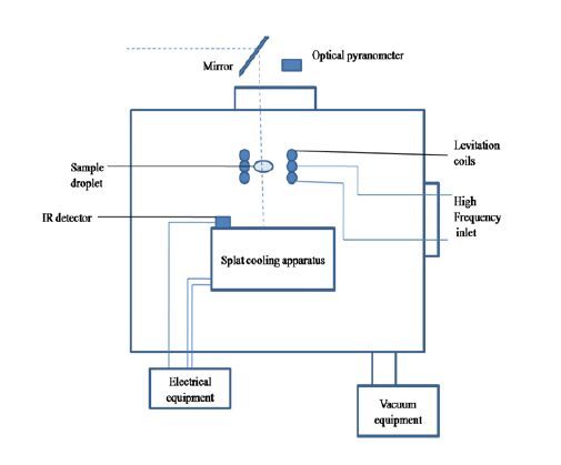
Futterer H, Wernhardt R, Pelzl J (1983) Splat cooling device for preparation of metallic glasses in inert gases. J Non-Cryst Solids 56: 435–438. doi: 10.1016/0022-3093(83)90508-2
![]() |
[35] |
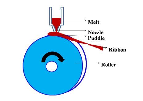
Budhani RC, Goel TC, Chopra KL (1982) Melt-Spining technique for preparation of metallic glass. Bull Mater Sci 4: 549–561. doi: 10.1007/BF02824962
![]() |
[36] |
Xu M, Ye Y, Morris JR (2006) Influence of Pd on formation of amorphous and quasicrystal phases in rapidly quenched Zr2Cu(1-x)Pdx. Philos Mag 86: 389–395 doi: 10.1080/14786430500300124
![]() |
[37] |
Limin W, Ma L, Inoue A (2003) Nanocrystal reinforced Hf60Ti15Ni5Cu10 metallic glass by melt spinning. J Alloy Compd 352: 265–269. doi: 10.1016/S0925-8388(02)01163-5
![]() |
[38] |
Schroers J, Quoc P, Amit D (2007) Thermoplastic forming of bulk metallic glass-A technology for MEMS and microstructure fabrication. J Microelectromech S 16: 240–247. doi: 10.1109/JMEMS.0007.892889
![]() |
[39] |
Ye JC, Chu JP, Chen YC (2012) Hardness, yield strength and plastic flow in thin film metallic-glass. J Appl Phys 112: 053516-053516-9. doi: 10.1063/1.4750028
![]() |
[40] | Wei B-H, Chu C-W, Huang C-H, et al. (2013) Characteristic studies on Zr-based metallic glass thin film on antibacterial capability fabricated by magnetron sputtering process. Bio Eng Res 3: 48–53. |
[41] | Liu Y, Liu J, Sohn S (2015) Metallic glass nanostructures of tunable shape and composition. Nat commun 6. |
[42] |
Santanu D, Santos-Ortiz R, Harpreet S (2016) Electromechanical behavior of pulsed laser deposited platinum-based metallic glass thin films. Physica Status Solidi 213: 399–404. doi: 10.1002/pssa.201532639
![]() |
[43] |
Wu X, Chen F, Zhang N, et al. (2016) Silver-Copper metallic glass electrocatalyst with high activity and stability comparable to Pt/C for Zinc-air batteries. J Mater Chem A 4: 3527–3537. doi: 10.1039/C5TA09266C
![]() |
[44] | Nagar S (2012) Multifunctional magnetic materials prepared by pulsed laser deposition. Doctoral dissertation. Department of material Science and Engineering, School of Industrial Engineering and Management, Royal Institute of technology ,Stockholm |
[45] | Saraf BM, Soodeh ZS (2013) Feasibility of Ti-based metallic glass coating in biomedical applications. Proceedings of 20th Iranian Conference on Biomedical Engineering (ICBME 2013), 18–20 December, University of Tehran, Tehran, Iran. |
[46] |
Ningshen S, Kamachi MU, Krishnan R (2011) Corrosion behavior of Zr-based metallic glass coating on type 304L stainless steel by pulsed laser deposition. Surf Coat Tech 205: 3961–3966. doi: 10.1016/j.surfcoat.2011.02.039
![]() |
[47] | Dapeng J (2010) Metal thin film growth on multi metallic surfaces: From quaternary metallic glass to binary crystal. Iowa State university. Graduate Theses. |
[48] |
Pookat G, Thomas H, Thomas S (2013) Evolution of structural and magnetic properties of Co-Fe based metallic glass thin films with thermal annealing. Surf Coat Tech 236: 246–251. doi: 10.1016/j.surfcoat.2013.09.055
![]() |
[49] |
Thomas S, Mathew J, Radhakrishnan P, et al. (2010) Metglas thin film based magnetostrictive transducers for use in long period fibre grating sensors. Sensor Actuat A-Phys 161: 83–90. doi: 10.1016/j.sna.2010.05.006
![]() |
[50] |
Chu JP, Lin CT, Mahalingam T (2004) Annealing induced full amorphisation in a multicomponent metallic film. Phys Rev B 69: 113410-1-4. doi: 10.1103/PhysRevB.69.113410
![]() |
[51] |
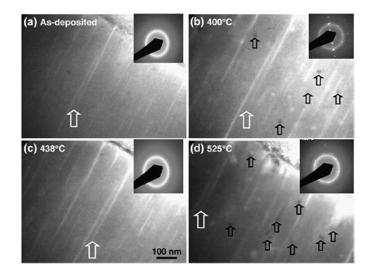
Chu JP, Wang C-Y, Chen LJ, et al. (2011) Annealing induced amorphisation in a sputtered glass forming film: In-situ transmission electron microscopy observation. Surf Coat Tech 205: 2914–2918. doi: 10.1016/j.surfcoat.2010.10.065
![]() |
[52] | Lin H-K, Lee C-J, Hu T-T, et al. (2012) Pulsed laser micromachining of Mg-Cu-Gd bulk metallic glass. Opt Laser Eng 50: 883–886. |
[53] | Williams E, Brousseau EB (2016) Nanosecond laser processing of Zr41.2Ti13.8Cu12.5Ni10Be22.5 with single pulses. J Mater Process Tech 232: 34–42. |
[54] | Cheung TL, Shek CH (2008) Surface characteristics of nitrogen and argon plasma immersion ion implantation of Cu-Zr-Al bulk metallic alloy. Rev Adv Mater Sci 18: 112–120. |
[55] |
Huang H-H, Huang H-M, Lin M-C, et al. (2014) Enhancing the bio-corossion resistance of Ni-free ZrCuFeAl bulk metallic glass through nitrogen plasma immersion ion implantation. J Alloy Compd 615: S660–S665. doi: 10.1016/j.jallcom.2014.01.098
![]() |
[56] |
Tam CY, Shek CH (2007) Improved oxidation resistance of Cu60Zr30Ti10 BMG with plasma immersion ion implantation. J Non-Cryst Solids 353: 3590–3595. doi: 10.1016/j.jnoncrysol.2007.05.118
![]() |
[57] |
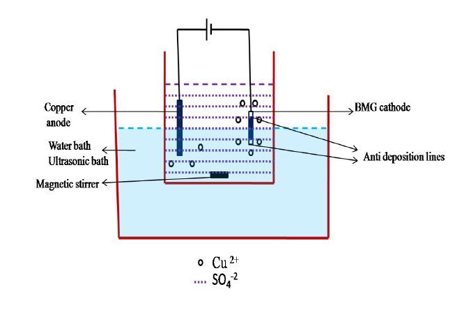
Qiu SB, Yao KF (2008) Novel application of the electrodeposition on bulk metallic glasses. Appl Surf Sci 255: 3454–3458. doi: 10.1016/j.apsusc.2008.07.077
![]() |
[58] |
Meng M, Gao Z, Ren L, et al. (2014). Improved plasticity of bulk metallic glasses by electrodeposition. Mater Sci Eng A 615: 240–246. doi: 10.1016/j.msea.2014.07.033
![]() |
[59] |
Turnbull D (1969) Under what conditions can a glass be formed. Contemp Phys 10: 473-488. doi: 10.1080/00107516908204405
![]() |
[60] | Inoue A, Koshiba H, Zhang T (1998) Wide supercooled liquid region and soft magnetic properties of Fe56Co7Ni7Zr0–10Nb (or Ta)0–10B20 amorphous alloys. J Appl Phys 83: 1967–1974 |
[61] |
Lu ZP, Liu CT (2002) A new glass forming ability criterion for bulk metallic glasses. J Acta Mater 50: 3501–3512. doi: 10.1016/S1359-6454(02)00166-0
![]() |
[62] |
Ji X, Ye P (2009) A thermodynamic approach to assess glass-forming ability of bulk metallic glasses. Trans Nonferrous Met Soc China 19: 1271–1279. doi: 10.1016/S1003-6326(08)60438-0
![]() |
[63] | Thompson CV, Spaepen F (1979) On the approximation of the free energy change of crystallization. Acta Metall 27: 1855–1859. |
[64] |
Mondal K, Murty BS (2005) On the parameters to assess the glass forming ability of liquids. J Non-Cryst Solids 351: 1366–1371. doi: 10.1016/j.jnoncrysol.2005.03.006
![]() |
[65] |
Ashmi TP, Arun P (2013) Study of glass transition kinetics for Co66Si12B16Fe4Mo2 metallic glass. Int J Mod Phys: Conference series 22: 321–326. doi: 10.1142/S2010194513010295
![]() |
[66] |
Lafi OA, Imran MMA (2011) Compositional dependence of thermal stability, glass forming ability and fragility index in some Se-Te-Sn glasses. J Alloys Compd 509: 5090–5094. doi: 10.1016/j.jallcom.2011.01.150
![]() |
[67] | Mukherjee S, Schroers J, Zhou Z (2004) Viscosity and specific volume of bulk metallic glass-forming alloys and their correlation with glass forming ability. Acta Mater 52: 3689–3695. |
[68] |
Daniel BM, Takeshi E, Katharine MF (2007). Structural aspects of Metallic Glasses. Mater Res soc Bulletin 32: 629–634. doi: 10.1557/mrs2007.124
![]() |
[69] |
Qin F, Wang X, Xie G, et al. (2007) Microstructure and corrosion resistance of Ti-Zr-Cu-Pd-Sn glassy and nanocrystalline alloys. Mater Trans 48: 167–170. doi: 10.2320/matertrans.48.167
![]() |
[70] | Laws KJ, Miracle DB, Ferry M (2015) A predictive structural model for bulk metallic glasses. Nat Commun 6: 1–10. |
[71] |
Sopu D, Albe K (2015) Influence of grain size and composition, topology and excess free volume on the deformation behavior of Cu-Zrnanoglasses. Beilstein J Nanotech 6: 537–545. doi: 10.3762/bjnano.6.56
![]() |
[72] |
Daniel BM (2004) A structural model for metallic glasses. Nat Mater 3: 697–702. doi: 10.1038/nmat1219
![]() |
[73] |
Wang K, Fujita T, Chen MW (2007) Electrical conductivity of a bulk metallic glass composite. Appl Phys Lett 91: 154101-1-154101-3. doi: 10.1063/1.2795800
![]() |
[74] |
Umetsu R Y, Tu R, Goto T (2012) Thermal and electrical transport properties of Zr-Based bulk metallic glassy alloys with high glass – forming ability. Mater Trans 53: 1721–1725. doi: 10.2320/matertrans.M2012163
![]() |
[75] | Dmitri VL, Larissa VL, Alexander YC (2013) Mechanical properties and deformation behavior of bulk metallic glasses. Metals 3: 1–22. |
[76] |
Zhang QS, Zhang W, Xie G, et al. (2010) Stable flowing of localised shear bands in soft bulk metallic glass. Acta Materialia 58: 904-909. doi: 10.1016/j.actamat.2009.10.005
![]() |
[77] |
Chen HS (1973) Plastic flow in metallic glasses under compression. Scr Metar 7: 931–935. doi: 10.1016/0036-9748(73)90143-9
![]() |
[78] |
Yu HB, Wang WH, Zhang JL (2009) Statistics analysis of the mechanical behavior of bulk metallic glasses. Adv Eng Mater 11: 370–375. doi: 10.1002/adem.200800380
![]() |
[79] | Daniel P, Yokoyama Y, Fujita K (2009) Correlation between structural relaxation and shear transformation zone volume of a bulk metallic glass. Appl Phys Lett 95: 141909-141909-3. |
[80] |
Louzguine DV, Kato H, Inoue A (2004) High-strength Cu-based cystal-glassy composite with enhanced ductility. Appl Phys Lett 84: 1088–1089. doi: 10.1063/1.1647278
![]() |
[81] |
Das J, Tang MB, Kim KB (2005) Work-hardenable ductile bulk metallic glass. Phys Rev Lett 94: 205501-1-205501-4. doi: 10.1103/PhysRevLett.94.205501
![]() |
[82] |
Hajlaoui K, Yavari AR, LeMoulec A (2007) Plasticity induced by nanoparticle dispersions in bulk metallic glasses. J Non-Cryst Solids 353: 327–331. doi: 10.1016/j.jnoncrysol.2006.10.011
![]() |
[83] | Saida J, Kato H, Setyawan ADH (2005) Characterisation and properties of nanocrystal-forming Zr-based bulk metallic glasses. Rev Adv Sci 10: 34–38. |
[84] |
Coddet P, Sanchette F, Rousset JC (2012) On the elastic modulus and hardness of co-sputtered Zr-Cu-(N) thin metal glass film. Surf Coat Tech 206: 3567–3571. doi: 10.1016/j.surfcoat.2012.02.036
![]() |
[85] |
Madoka O, Kyoko N, Ryuji T (2005) Tungsten-based metallic glasses with high crystallisation temperature, high modulus and high hardness. Mater Trans 46: 48–53. doi: 10.2320/matertrans.46.48
![]() |
[86] |
Inoue A (2000) Stabilization of metallic supercooled liquid and bulk amorphous alloys. Acta Mater 48: 279–306. doi: 10.1016/S1359-6454(99)00300-6
![]() |
[87] |
Ye JC, Lu J, Yang Y, et al. (2010) Extraction of bulk metallic glass yield strengths using tapered micropillars in micro compression experiments. Intermetallics 18: 385–393. doi: 10.1016/j.intermet.2009.08.011
![]() |
[88] |
Chou HS, Huang JC, Chang LW (2008) Structural relaxation and nanoindentation response in Zr-Cu-Ti amorphous thin films. Appl Phys Lett 93: 191901-1-191901-3. doi: 10.1063/1.2999592
![]() |
[89] |
Chou HS, Huang JC, Chang LW (2010) Mechanical properties of ZrCuTi thin film metallic glass with high content of immiscible tantalum. Surf Coat Tech 205: 587–590. doi: 10.1016/j.surfcoat.2010.07.042
![]() |
[90] | Johnson WL, Samwer K (2005) A universal criterion for plastic yielding of metallic glasses with a (T/Tg)2/3 temperature dependence. Phys Rev Lett 95: 195501. |
[91] |
Blau PJ (2001) Friction and wear of Zr-based amorphous metal alloy under dry and lubricated conditions. Wear 250: 431–434. doi: 10.1016/S0043-1648(01)00627-5
![]() |
[92] | Fu XY, Kasai T, Falk ML (2001) Sliding behavior of metallic glass – Part I. Experimental Investigations. Wear 250: 409–419. |
[93] |
Zeynep P, Mustafa B, Albert JS (2008) Sliding tribological characteristics of Zr-based bulk metallic glass. Intermetallics 16: 34–41. doi: 10.1016/j.intermet.2007.07.011
![]() |
[94] |
Tam CY, Shek CH (2004) Abrasive wear of Cu60Zr30Ti10 bulk metallic glass. Mater Sci Eng A 384: 138–142. doi: 10.1016/j.msea.2004.05.073
![]() |
[95] |
Prakash B (2005) Abrasive behavior of Fe, Co and Ni based metallic glasses. Wear 258: 217–224. doi: 10.1016/j.wear.2004.09.010
![]() |
[96] | Bhushan B (2002) Introduction to tribology. John Wiley and Sons. |
[97] |
Jang B-T, Yi S-H, Kim S-S (2010) Tribological behavior of Fe-based bulk metallic glass. J Mech Sci Technol 24: 89–92. doi: 10.1007/s12206-009-1123-8
![]() |
[98] | Liu FX, Yang FQ, Gao YF (2009) Micro-scratch study of a magnetron-sputtered Zr-based metallic-glass film. Surf Coat Tech 203: 3480–3484. |
[99] | Chunling Q, Katsuhiko A, Tao Z (2003) Corrosion behavior of Cu-Zr-Ti-Nb bulk glassy alloys. Mater Trans 4: 749–753. |
[100] |
Qin F, Yoshimura M, Wang X, et al. (2007) Corrosion behavior of a Ti-based bulk metallic glass and its crystalline alloys. Mater Trans 48: 1855–1858. doi: 10.2320/matertrans.MJ200713
![]() |
[101] |
Vincent S, Khan AF, Murty BS (2013) Corrosion characterization on melt spun Cu60Zr20Ti20 metallic glass: An experimental case study. J Non-Cryst Solids 379: 48–53. doi: 10.1016/j.jnoncrysol.2013.07.007
![]() |
[102] |
Chen L-T, Lee J-W, Yang Y-C, et al. (2014) Microstructure, mechanical and anti-corrosion property evaluation of iron-based thin film metallic glasses. Surf Coat Tech 260: 46–55. doi: 10.1016/j.surfcoat.2014.07.039
![]() |
[103] |
Inoue A, Shinohara Y, Gook JS (1995) Thermal and magnetic properties of bulk Fe-based glassy alloys prepared by copper mold casting. Mater Trans 36: 1427-1433. doi: 10.2320/matertrans1989.36.1427
![]() |
[104] |
Inoue A, Zhang T, Zhang W, et al. (1996) Bulk Nd-Fe-Al amorphous alloys with hard magnetic properties. Mater Trans 37: 99-108. doi: 10.2320/matertrans1989.37.99
![]() |
[105] | Boll R, Weichmagnetische W, GmbH VAC (1990) Siemens AG Berlin und München, Germany. |
[106] |
Chu JP, Lo CT, Fang YK, et al. (2006) On annealing-induced amorphisation and anisotropy in a ferromagnetic Fe-based film: a magnetic and property study. Appl Phys Lett 88: 012510-1-012510-3. doi: 10.1063/1.2161938
![]() |
[107] |
Wahyu D, Jinn PC, Berhanu TK (2015) Thin film metallic glasses in optoelectronic, magnetic and electronic applications: A recent update. Curr Opin Solid State Mater Sci 19: 95–106. doi: 10.1016/j.cossms.2015.01.001
![]() |
[108] |
Kim H, Gilmore CM, Pique A (1999) Electrical, optical and structural properties of indium-tin-oxide thin films for organic light-emitting devices. J Appl Phys 86: 6451–6461. doi: 10.1063/1.371708
![]() |
[109] |
Hu TT, Hsu J, Huang JC (2012) Correlation between reflectivity and resistivity in multi component metallic systems. Appl Phys Lett 101: 011902-1-011902-4. doi: 10.1063/1.4732143
![]() |
[110] | Chen H-W, Hsu K-C, Chan Y-C, et al. (2014) Antimicrobial properties of Zr-Cu-Al-Ag thin film metallic glass. Thin Solid Films 561: 98–101. |
[111] | Weissman Z, Berdicevsky I, Cavari BZ (2000) The high copper tolerance of Candida albicans is mediated by a P-type ATPase. P Nati Acad Sci USA 28: 3520–3525. |
[112] |
Chu JP, Tz-Yah L, Chia-Lin L (2014) Fabrication and characterisations of thin film metallic glasses: Antibacterial property and durability study for medical application. Thin Solid Films 561: 102–107 doi: 10.1016/j.tsf.2013.08.111
![]() |
[113] |
Chu YY, Lin YS, Chang CM (2014) Promising antimicrobial capability of thin film metallic glasses. Mater Sci Eng C 36: 221–225. doi: 10.1016/j.msec.2013.12.015
![]() |
[114] |
Sharma P, Kaushik N, Kimura H (2007) Nano-fabrication with metallic glass – An exotic material for nano-electromechanical systems. Nanotechnology 18: 035302-1-035302-6. doi: 10.1088/0957-4484/18/3/035302
![]() |
[115] |
Trukenmuller R, Giselbrecht S, Rivron N (2011) Thermoforming of film-based biomedical microdevices. Adv Mater 23: 1311–1329. doi: 10.1002/adma.201003538
![]() |
[116] |
Kaushik N, Sharma P, Ahadian S (2014) Metallic glass thin films for potential biomedical applications. J Biomed Mater Res Part B 102: 1544–1552. doi: 10.1002/jbm.b.33135
![]() |
[117] | Felix G, Klaus V, Wei-Shan W (2015) Towards MEMS loudspeaker fabrication by using metallic glass thin films. Fraunhofer Institute for Electronic Nano Systems ENAS. Available from: http://www.enas.fraunhofer.de/content/- |
[118] | Seiichi H, Junpei S, Akira S (2005) Thin film metallic glasses as new MEMS materials. IEEE International Conference on Micro Electro Mechanical Systems. |
[119] |
Junpei S, Seiichi H (2015) Characteristics of Ti-Ni-Zr thin film metallic glasses/thin film shape memory alloys for micro actuators with three dimensional structures. Int J Autom Tech 9: 662–667. doi: 10.20965/ijat.2015.p0662
![]() |
[120] |
Susumu K, Shin-ichi Y, Hisamichi K (2010) Composition control of Pd-Cu-Si metallic glassy alloys for thin film hydrogen sensor. Mater Trans 51: 2133–2138. doi: 10.2320/matertrans.M2010254
![]() |
[121] |
Ishida M, Takeda H, Watanabe D (2004) Fillability and imprintability of high strength Ni-based bulk metallic glass prepared by the precision Die-casting technique. Mater Trans 45: 1239–1244. doi: 10.2320/matertrans.45.1239
![]() |
[122] | Inoue A, Wang XM, Zhang W (2008) Developments and applications of bulk metallic glasses. Rev Adv Mater Sci 18: 1–9. |
1. | OlaOluwa S. Yaya, Hammed A. Olayinka, Ahamuefula E. Ogbonna, Mamdouh Abdulaziz Saleh Al-Faryan, Xuan Vinh Vo, Dynamic connectedness of economic policy uncertainty in G7 countries and the influence of the USA and UK on non-G7 countries, 2024, 57, 1573-9414, 10.1007/s10644-024-09658-1 | |
2. | OlaOluwa S. Yaya, Dynamic connectedness of Economic Policy Uncertainty in G7 countries, and the influence of the US and UK on non-G7 countries, 2024, 1556-5068, 10.2139/ssrn.4794166 | |
3. | Naveed Khan, OlaOluwa S. Yaya, Xuan Vinh Vo, Hassan Zada, Quantile time-frequency connectedness and spillovers among financial stress, cryptocurrencies and commodities, 2025, 103, 03014207, 105527, 10.1016/j.resourpol.2025.105527 |
Min | Mean | Median | SD | Max | |
Gbp | 1.149 | 1.533 | 1.534 | 0.222 | 2.108 |
Eur | 1.039 | 1.258 | 1.261 | 0.128 | 1.599 |
Jpy | 75.740 | 103.565 | 107.164 | 12.768 | 125.629 |
Aud | 0.574 | 0.829 | 0.783 | 0.120 | 1.103 |
Cny | 6.031 | 6.696 | 6.652 | 0.453 | 8.022 |
Series | No terms | Intercept only | Intercept with time trend |
GBP | 0.153 (0.134, 0.172) | 0.153 (0.134, 0.172) | 0.152 (0.133, 0.171) |
EUR | 0.243 (0.218, 0.268) | 0.243 (0.218, 0.268) | 0.240 (0.215, 0.265) |
JPY | 0.238 (0.214, 0.262) | 0.238 (0.214, 0.262) | 0.234 (0.209, 0.259) |
AUD | 0.201 (0.182, 0.220) | 0.201 (0.182, 0.220) | 0.198 (0.179, 0.217) |
CNY | 0.186 (0.142, 0.230) | 0.186 (0.142, 0.230) | 0.182 (0.138, 0.226) |
Note: in bold are selected results obtained based on the significance of parameters of the deterministic terms in Robinson's (1994) framework. |
Pairs | m = T0.5 | m = T0.6 |
GBP – EUR | 1.610 | 0.003 |
GBP – JPY | 0.757 | 0.073 |
GBP – AUD | 0.289 | 1.677 |
GBP – CNY | 0.005 | 0.196 |
EUR – JPY | 0.998 | 0.090 |
EUR – AUD | 1.355 | 1.640 |
EUR – CNY | 1.596 | 0.191 |
JPY – AUD | 0.499 | 1.722 |
JPY – CNY | 0.749 | 0.267 |
AUD – CNY | 0.265 | 1.382 |
Note: The homogeneity of fractional d is distributed normally, therefore the two-sided critical point is 1.96 at a 5% level. |
Pairs | m = T0.5 | m = T0.6 |
GBP – EUR | 0.492 | 0.415 |
GBP – JPY | 0.468 | 0.368 |
GBP – AUD | 0.423 | 0.418 |
GBP – CNY | 0.153 | 0.189 |
EUR – JPY | 0.720 | 0.703 |
EUR – AUD | 0.622 | 0.598 |
EUR – CNY | −0.401 | −0.212 |
JPY – AUD | 0.567 | 0.553 |
JPY – CNY | −0.309 | −0.187 |
AUD – CNY | −0.512 | −0.321 |
Pairs | m = T0.5 | m = T0.6 |
GBP – EUR | 0.141 (0.118, 0.163) | 0.137 (0.114, 0.159) |
GBP – JPY | 0.129 (0.107, 0.150) | 0.127 (0.105, 0.149) |
GBP – AUD | 0.087 (0.066, 0.108) | 0.087 (0.067, 0.108) |
GBP – CNY | 0.152 (0.133, 0.171) | 0.152 (0.133, 0.171) |
EUR – JPY | 0.144 (0.123, 0.166) | 0.146 (0.124, 0.168) |
EUR – AUD | 0.181 (0.153, 0.208) | 0.184 (0.156, 0.211) |
EUR – CNY | 0.243 (0.218, 0.268) | 0.243 (0.218, 0.268) |
JPY – AUD | 0.178 (0.152, 0.203) | 0.179 (0.154, 0.205) |
JPY – CNY | 0.238 (0.214, 0.262) | 0.238 (0.214, 0.262) |
AUD – CNY | 0.201 (0.182, 0.220) | 0.201 (0.182, 0.220) |
Pairs | y1t - y2t | Residual-based fractional cointegration test | |
m = T0.5 | m = T0.6 | ||
GBP – EUR | 0.153 - 0.243 | 0.141* | 0.137* |
GBP – JPY | 0.153 - 0.238 | 0.129* | 0.127* |
GBP – AUD | 0.153 - 0.198 | 0.087* | 0.087* |
GBP – CNY | 0.153 - 0.186 | 0.152* | 0.152* |
EUR – JPY | 0.243 - 0.238 | 0.144* | 0.146* |
EUR – AUD | 0.243 - 0.198 | 0.181* | 0.184* |
EUR – CNY | 0.243 - 0.186 | 0.243 | 0.243 |
JPY – AUD | 0.238 - 0.198 | 0.178* | 0.179* |
JPY – CNY | 0.238 - 0.186 | 0.238 | 0.238 |
AUD – CNY | 0.198 - 0.186 | 0.201 | 0.201 |
Note: in bold and * indicates cases of de<min(dy1,dy2). |
Pairs | NET | TCIτ | |
y1t | y2t | ||
GBP – EUR | Transmitter | Receiver | 27.88 |
GBP – JPY | Transmitter | Receiver | 12.71 |
GBP – AUD | Receiver | Transmitter | 24.59 |
GBP – CNY | Transmitter | Receiver | 6.20 |
EUR – JPY | Transmitter | Receiver | 22.13 |
EUR – AUD | Receiver | Transmitter | 25.61 |
EUR – CNY | Transmitter | Receiver | 7.61 |
JPY – AUD | Transmitter | Receiver | 15.77 |
JPY – CNY | Transmitter | Receiver | 6.00 |
AUD – CNY | Transmitter | Receiver | 6.20 |
Pairs | NET | TCIτ | |
y1t | y2t | ||
GBP – EUR | Receiver | Transmitter | 63.72 |
GBP – JPY | Undecided | Undecided | 53.69 |
GBP – AUD | Transmitter | Receiver | 64.00 |
GBP – CNY | Receiver | Transmitter | 39.55 |
EUR – JPY | Transmitter | Receiver | 60.01 |
EUR – AUD | Transmitter | Receiver | 63.28 |
EUR – CNY | Receiver | Transmitter | 39.69 |
JPY – AUD | Receiver | Transmitter | 56.81 |
JPY – CNY | Receiver | Transmitter | 38.33 |
AUD – CNY | Receiver | Transmitter | 41.79 |
Pairs | NET | TCIτ | |
y1t | y2t | ||
GBP – EUR | Transmitter | Receiver | 84.64 |
GBP – JPY | Receiver | Transmitter | 82.36 |
GBP – AUD | Receiver | Transmitter | 85.63 |
GBP – CNY | Receiver | Transmitter | 80.09 |
EUR – JPY | Transmitter | Receiver | 83.13 |
EUR – AUD | Receiver | Transmitter | 85.74 |
EUR – CNY | Receiver | Transmitter | 80.71 |
JPY – AUD | Transmitter | Receiver | 83.15 |
JPY – CNY | Receiver | Transmitter | 80.28 |
AUD – CNY | Receiver | Transmitter | 81.41 |
Pairs | wijt | βijt |
GBP - AUD | 0.73 | 0.42 |
GBP - CNY | 0.07 | 0.40 |
GBP - EUR | 0.53 | 0.58 |
GBP – JPY | 0.54 | 0.14 |
EUR - AUD | 0.70 | 0.42 |
EUR - CNY | 0.09 | 0.60 |
EUR – GBP | 0.47 | 0.61 |
EUR – JPY | 0.53 | 0.21 |
AUD - CNY | 0.04 | 0.73 |
AUD - EUR | 0.30 | 0.64 |
AUD- GBP | 0.27 | 0.69 |
AUD – JPY | 0.42 | 0.10 |
CNY - AUD | 0.96 | 0.07 |
CNY - EUR | 0.91 | 0.08 |
CNY - GBP | 0.93 | 0.06 |
CNY – JPY | 0.89 | 0.03 |
JPY – AUD | 0.58 | 0.08 |
JPY - CNY | 0.11 | 0.16 |
JPY – EUR | 0.47 | 0.23 |
JPY – GBP | 0.46 | 0.14 |