Geopolymer materials have emerged as promising alternatives to ordinary Portland cementitious materials, offering more sustainable solutions for concrete production. Sodium aluminosilicate hydrate (N-A-S-H) serves as a crucial component in geopolymer concrete, while its thermomechanical properties at elevated temperatures remain relatively underexplored. This study examined the molecular structural variations of N-A-S-H within a temperature range of 300–900 K. The influence of different Si/Al ratios and temperature levels on molecular characteristics and atomic mobility was analyzed using the radial distribution function (RDF) and mean square displacement (MSD). The thermal conductivity of the N-A-S-H gel was determined using the Müller-Plathe reverse nonequilibrium molecular dynamics (RNEMD) method. Results show that as temperature increases, the mobility of Si and Al atoms is enhanced, and the thermal conductivity of N-A-S-H gel ranges from 1.431 to 1.857 W/m/K. The thermal conductivity increases with higher Si/Al ratios and elevated temperatures, suggesting decreased thermal insulation performance at higher Si/Al ratios and temperatures.
Citation: Yun-Lin Liu, Si-Yu Ren, Dong-Hua Wang, Ding-Wei Yang, Ming-Feng Kai, Dong Guo. Molecular structure and thermal conductivity of hydrated sodium aluminosilicate (N-A-S-H) gel under different Si/Al ratios and temperatures: A molecular dynamics analysis[J]. AIMS Materials Science, 2025, 12(2): 258-277. doi: 10.3934/matersci.2025014
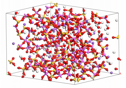
Geopolymer materials have emerged as promising alternatives to ordinary Portland cementitious materials, offering more sustainable solutions for concrete production. Sodium aluminosilicate hydrate (N-A-S-H) serves as a crucial component in geopolymer concrete, while its thermomechanical properties at elevated temperatures remain relatively underexplored. This study examined the molecular structural variations of N-A-S-H within a temperature range of 300–900 K. The influence of different Si/Al ratios and temperature levels on molecular characteristics and atomic mobility was analyzed using the radial distribution function (RDF) and mean square displacement (MSD). The thermal conductivity of the N-A-S-H gel was determined using the Müller-Plathe reverse nonequilibrium molecular dynamics (RNEMD) method. Results show that as temperature increases, the mobility of Si and Al atoms is enhanced, and the thermal conductivity of N-A-S-H gel ranges from 1.431 to 1.857 W/m/K. The thermal conductivity increases with higher Si/Al ratios and elevated temperatures, suggesting decreased thermal insulation performance at higher Si/Al ratios and temperatures.

| [1] |
Hayat U, Kai MF, A HB, et al. (2024) Atomic-level investigation into the transport of NaCl solution in porous cement paste: The effects of pore size and temperature. J Build Eng 86: 108976. https://doi.org/10.1016/j.jobe.2024.108976 doi: 10.1016/j.jobe.2024.108976

|
| [2] |
Liu YL, Li CF, Zhai HX, et al. (2023) Production and performance of CO2 modified foam concrete. Constr Build Mater 389: 131671. https://doi.org/10.1016/j.conbuildmat.2023.131671 doi: 10.1016/j.conbuildmat.2023.131671
|
| [3] |
Maddalena R, Roberts JJ, Hamilton A, et al. (2018) Can Portland cement be replaced by low-carbon alternative materials? A study on the thermal properties and carbon emissions of innovative cements. J Clean Prod 186: 933–942. https://doi.org/10.1016/j.jclepro.2018.02.138 doi: 10.1016/j.jclepro.2018.02.138
|
| [4] |
Chairunnisa N, Haryanti NH, Nurwidayati R, et al. (2024) Characteristics of metakaolin-based geopolymers using bemban fiber additives. AIMS Mater Sci 11: 815–832. https://doi.org/10.3934/matersci.2024040 doi: 10.3934/matersci.2024040
|
| [5] |
Liu Y, Huo S, Fu J, et al. (2024) Dynamic properties of CO2-cured foam concrete at different loading rates: Effect of the foam admixtures and addition of polypropylene fiber. Front Mater 11: 1445848. https://doi.org/10.3389/fmats.2024.1445848 doi: 10.3389/fmats.2024.1445848
|
| [6] |
Hassan A, Arif M, Shariq M, et al. (2022) Fire resistance characteristics of geopolymer concrete for environmental sustainability: A review of thermal, mechanical and microstructure properties. Environ Dev Sustain 25: 8975–9010. https://doi.org/10.1007/s10668-022-02495-0 doi: 10.1007/s10668-022-02495-0
|
| [7] |
He R, Dai N, Wang Z, et al. (2020) Thermal and mechanical properties of geopolymers exposed to high temperature: A literature review. Adv Civ Eng 2020: 7532703. https://doi.org/10.1155/2020/7532703 doi: 10.1155/2020/7532703
|
| [8] |
Habert G, De Lacaillerie JB, Roussel N, et al. (2011) An environmental evaluation of geopolymer based concrete production: Reviewing current research trends. J Clean Prod 19: 1229–1238. https://doi.org/10.1016/j.jclepro.2011.03.012 doi: 10.1016/j.jclepro.2011.03.012
|
| [9] |
Mahmoud HA, Tawfik TA, Abd El-razik MM, et al. (2023) Mechanical and acoustic absorption properties of lightweight fly ash/slag-based geopolymer concrete with various aggregates. Ceram Int 49: 21142–21154. https://doi.org/10.1016/j.ceramint.2023.03.244 doi: 10.1016/j.ceramint.2023.03.244
|
| [10] |
Mathew G, Issac BM (2020) Effect of molarity of sodium hydroxide on the aluminosilicate content in laterite aggregate of laterised geopolymer concrete. J Build Eng 32: 101486. https://doi.org/10.1016/j.jobe.2020.101486 doi: 10.1016/j.jobe.2020.101486
|
| [11] |
Liu YL, Liu C, Qian LP, et al. (2023) Foaming processes and properties of geopolymer foam concrete: Effect of the activator. Constr Build Mater 391: 131830. https://doi.org/10.1016/j.conbuildmat.2023.131830 doi: 10.1016/j.conbuildmat.2023.131830
|
| [12] |
Duxson P, Fernández-Jiménez A, Provis JL, et al. (2006) Geopolymer technology: The current state of the art. J Mater Sci 42: 2917–2933. http://dx.doi.org/10.1007/s10853-006-0637-z doi: 10.1007/s10853-006-0637-z
|
| [13] |
Li W, Wang Y, Yu C, et al. (2022) Nano-scale study on molecular structure, thermal stability, and mechanical properties of geopolymer. J Korean Ceram Soc 60: 413–423. https://doi.org/10.1007/s43207-022-00276-z doi: 10.1007/s43207-022-00276-z
|
| [14] |
Shang J, Dai JG, Zhao TJ, et al. (2018) Alternation of traditional cement mortars using fly ash-based geopolymer mortars modified by slag. J Clean Prod 203: 746–756. https://doi.org/10.1016/j.jclepro.2018.08.255 doi: 10.1016/j.jclepro.2018.08.255
|
| [15] |
Lemougna PN, Adediran A, Yliniemi J, et al. (2020) Thermal stability of one-part metakaolin geopolymer composites containing high volume of spodumene tailings and glass wool. Cem Concr Compos 114: 103792. https://doi.org/10.1016/j.cemconcomp.2020.103792 doi: 10.1016/j.cemconcomp.2020.103792
|
| [16] |
Cheng TW, Chiu JP (2003) Fire-resistant geopolymer produced by granulated blast furnace slag. Miner Eng 16: 205–210. https://doi.org/10.1016/S0892-6875(03)00008-6 doi: 10.1016/S0892-6875(03)00008-6
|
| [17] |
Amran M, Huang SS, Debbarma S, et al. (2022) Fire resistance of geopolymer concrete: A critical review.Constr Build Mater 324: 126722. https://doi.org/10.1016/j.conbuildmat.2022.126722 doi: 10.1016/j.conbuildmat.2022.126722
|
| [18] |
Temuujin J, Minjigmaa A, Rickard W, et al. (2010) Fly ash based geopolymer thin coatings on metal substrates and its thermal evaluation. J Hazard Mater 180: 748–752. https://doi.org/10.1016/j.jhazmat.2010.04.121 doi: 10.1016/j.jhazmat.2010.04.121
|
| [19] |
Abdolhosseini Qomi MJ, Ulm FJ, Pellenq RJM (2015) Physical origins of thermal properties of cement paste. Phys Rev Appl 3: 064010. https://doi.org/10.1103/PhysRevApplied.3.064010 doi: 10.1103/PhysRevApplied.3.064010
|
| [20] |
Liu W, Ju S (2024) Tunable thermal conductivity of sustainable geopolymers by the Si/Al ratio and moisture content: Insights from atomistic simulations. J Phys Chem B 128: 2972–2984. https://doi.org/10.1021/acs.jpcb.3c07445 doi: 10.1021/acs.jpcb.3c07445
|
| [21] |
Kamseu E, Ceron B, Tobias H, et al. (2011) Insulating behavior of metakaolin-based geopolymer materials assess with heat flux meter and laser flash techniques. J Therm Anal Calorim 108: 1189–1199. https://doi.org/10.1007/s10973-011-1798-9 doi: 10.1007/s10973-011-1798-9
|
| [22] |
Akbulut ZF, Guler S, Khan M, et al. (2023) The effects of waste iron powder and steel fiber on the physical and mechanical properties of geopolymer mortars exposed to high temperatures. Structures 58: 105398. https://doi.org/10.1016/j.istruc.2023.105398 doi: 10.1016/j.istruc.2023.105398
|
| [23] |
Samal S, Phan Thanh N, Petríková I, et al. (2015) Improved mechanical properties of various fabric-reinforced geocomposite at elevated temperature. JOM 67: 1478–1485. https://doi.org/10.1007/s11837-015-1420-x doi: 10.1007/s11837-015-1420-x
|
| [24] |
Wang J, Chen X, Li C, et al. (2023) Evaluating the effect of kaliophilite on the fire resistance of geopolymer concrete. J Build Eng 75: 106975. https://doi.org/10.1016/j.jobe.2023.106975 doi: 10.1016/j.jobe.2023.106975
|
| [25] |
Kupwade-Patil K, Soto F, Kunjumon A, et al. (2013) Multi-scale modeling and experimental investigations of geopolymeric gels at elevated temperatures. Comput Struct 122: 164–177. https://doi.org/10.1016/j.compstruc.2013.01.005 doi: 10.1016/j.compstruc.2013.01.005
|
| [26] |
Kong DL, Sanjayan JG, Sagoe-Crentsil K, et al. (2007) Factors affecting the performance of metakaolin geopolymers exposed to elevated temperatures. J Mater Sci 43: 824–831. https://doi.org/10.1007/s10853-007-2205-6 doi: 10.1007/s10853-007-2205-6
|
| [27] |
Cai J, Li X, Tan J, et al. (2020) Thermal and compressive behaviors of fly ash and metakaolin-based geopolymer. J Build Eng 30: 101307. https://doi.org/10.1016/j.jobe.2020.101307 doi: 10.1016/j.jobe.2020.101307
|
| [28] |
Agustini NKA, Triwiyono A, Sulistyo D, et al. (2020) Effects of water to solid ratio on thermal conductivity of fly ash-based geopolymer paste. IOP Conf Ser Earth Environ Sci 426: 012010. https://doi.org/10.1088/1755-1315/426/1/012010 doi: 10.1088/1755-1315/426/1/012010
|
| [29] |
Pan Z, Tao Z, Cao YF, et al. (2018) Compressive strength and microstructure of alkali-activated fly ash/slag binders at high temperature. Cem Concr Compos 86: 9–18. https://doi.org/10.1016/j.cemconcomp.2017.09.011 doi: 10.1016/j.cemconcomp.2017.09.011
|
| [30] |
Wang P, Zhang Q, Wang M, et al. (2019) Atomistic insights into cesium chloride solution transport through the ultra-confined calcium–silicate–hydrate channel. Phys Chem Chem Phys 21: 11892–11902. https://doi.org/10.1039/C8CP07676F doi: 10.1039/C8CP07676F
|
| [31] |
Chen Y, de Lima LM, Li Z, et al. (2024). Synthesis, solubility and thermodynamic prperties of NASH gels with various target Si/Al ratios. Cem Concr Res 180: 107484. https://doi.org/10.1016/j.cemconres.2024.107484 doi: 10.1016/j.cemconres.2024.107484
|
| [32] |
Zhang W, Lang L, Chen X, et al. (2024) Adsorption mechanism of Cs+ and Pb2+ on the NASH surface under the different Si/Al ratio and temperature. J Mol Liq 40: 124558. https://doi.org/10.1016/j.molliq.2024.124558 doi: 10.1016/j.molliq.2024.124558
|
| [33] |
He Y, Savic I, Donadio D, et al. (2012) Lattice thermal conductivity of semiconducting bulk materials: Atomistic simulations. Phys Chem Chem Phys 14: 16209–16222. https://doi.org/10.1039/C2CP42394D doi: 10.1039/C2CP42394D
|
| [34] |
Yousefi F, Khoeini F, Rajabpour A, et al. (2020) Thermal conductivity and thermal rectification of nanoporous graphene: A molecular dynamics simulation. Int J Heat Mass Transf 146: 118884. https://doi.org/10.1016/j.ijheatmasstransfer.2019.118884 doi: 10.1016/j.ijheatmasstransfer.2019.118884
|
| [35] |
Zhang X, Xie H, Hu M, et al. (2014) Thermal conductivity of silicene calculated using an optimized Stillinger-Weber potential. Phys Rev B 89: 054310. https://doi.org/10.1103/PhysRevB.89.054310 doi: 10.1103/PhysRevB.89.054310
|
| [36] |
Zhang X, Zhang J, Yang M, et al. (2020) Molecular dynamics study on the thermal conductivity of bilayer graphene with nitrogen doping. Solid State Commun 309: 113845. https://doi.org/10.1016/j.ssc.2020.113845 doi: 10.1016/j.ssc.2020.113845
|
| [37] |
Che J, Çağın T, Deng W, et al. (2000) Thermal conductivity of diamond and related materials from molecular dynamics simulations. J Chem Phys 113: 6888–6900. https://doi.org/10.1063/1.1310223 doi: 10.1063/1.1310223
|
| [38] |
Jund P, Jullien R (1999) Molecular-dynamics calculation of the thermal conductivity of vitreous silica. Phys Rev B 59: 13707–13711. https://doi.org/10.1103/PhysRevB.59.13707 doi: 10.1103/PhysRevB.59.13707
|
| [39] |
Tretiakov KV, Scandolo S (2004) Thermal conductivity of solid argon at high pressure and high temperature: A molecular dynamics study. J Chem Phys 121: 11177–11182. https://doi.org/10.1063/1.1812754 doi: 10.1063/1.1812754
|
| [40] |
Esfarjani K, Chen G, Stokes HT, et al. (2011) Heat transport in silicon from first-principles calculations. Phys Rev B 84: 085204. https://doi.org/10.1103/PhysRevB.84.085204 doi: 10.1103/PhysRevB.84.085204
|
| [41] |
Schelling PK, Phillpot SR, Keblinski P, et al. (2002) Comparison of atomic-level simulation methods for computing thermal conductivity. Phys Rev B 65: 144306. https://doi.org/10.1103/PhysRevB.65.144306 doi: 10.1103/PhysRevB.65.144306
|
| [42] |
Müller-Plathe F (1997) A simple nonequilibrium molecular dynamics method for calculating the thermal conductivity. J Chem Phys 106: 6082–6085. https://doi.org/10.1063/1.473271 doi: 10.1063/1.473271
|
| [43] |
Du H, Shi J, Chen Z, et al. (2022) Reverse nonequilibrium molecular dynamics simulation for thermal conductivity of gallium-based liquid metal. J Phys Chem C 126: 20558–20569. https://doi.org/10.1021/acs.jpcc.2c04023 doi: 10.1021/acs.jpcc.2c04023
|
| [44] |
Loulijat H, Moustabchir H (2021) A study of the effects of graphene nanosheets on the thermal conductivity of nanofluid (argon-graphene) using reverse nonequilibrium molecular dynamics method. Int J Thermophys 42: 125. https://doi.org/10.1007/s10765-021-02877-y doi: 10.1007/s10765-021-02877-y
|
| [45] |
Zhu M, Li J, Chen J, et al. (2019) Improving thermal conductivity of epoxy resin by filling boron nitride nanomaterials: A molecular dynamics investigation. Comput Mater Sci 164: 108–115. https://doi.org/10.1016/j.commatsci.2019.04.012 doi: 10.1016/j.commatsci.2019.04.012
|
| [46] |
Zhang C, Hao XL, Wang CX, et al. (2017) Thermal conductivity of graphene nanoribbons under shear deformation: A molecular dynamics simulation. Sci Rep 7: 41398. https://doi.org/10.1038/srep41398 doi: 10.1038/srep41398
|
| [47] | Shabib I, Abu-Shams M, Khan MR, et al. (2014) Lattice thermal conductivity of Fe-Cr alloys with < 001 > tilt boundaries: An atomistic study. Proceedings of the ASME 2014 International Mechanical Engineering Congress and Exposition. Volume 9: Mechanics of Solids, Structures and Fluids. Montreal, Quebec, Canada. https://doi.org/10.1115/IMECE2014-38408 |
| [48] |
Wan H, Yuan L, Zhang Y, et al. (2020) Insight into the leaching of sodium alumino-silicate hydrate (N-A-S-H) gel: A molecular dynamics study. Front Mater 7: 56. https://doi.org/10.3389/fmats.2020.00056 doi: 10.3389/fmats.2020.00056
|
| [49] |
Tian Z, Zhang Z, Tang X, et al. (2023) Understanding the effect of moisture on interfacial behaviors of geopolymer-aggregate interaction at molecular level. Constr Build Mater 385: 131404. https://doi.org/10.1016/j.conbuildmat.2023.131404 doi: 10.1016/j.conbuildmat.2023.131404
|
| [50] |
Wang R, Wang J, Dong T, et al. (2020) Structural and mechanical properties of geopolymers made of aluminosilicate powder with different SiO2/Al2O3 ratio: Molecular dynamics simulation and microstructural experimental study. Constr Build Mater 240: 117935. https://doi.org/10.1016/j.conbuildmat.2019.117935 doi: 10.1016/j.conbuildmat.2019.117935
|
| [51] |
Wang R, Wang J, Song Q, et al. (2021) The effect of Na+ and H2O on structural and mechanical properties of coal gangue-based geopolymer: Molecular dynamics simulation and experimental study. Constr Build Mater 268: 121081. https://doi.org/10.1016/j.conbuildmat.2020.121081 doi: 10.1016/j.conbuildmat.2020.121081
|
| [52] |
Bagheri A, Nazari A, Sanjayan JG, et al. (2018) Molecular simulation of water and chloride ion diffusion in nanopores of alkali-activated aluminosilicate structures. Ceram Int 44: 20723–20731. https://doi.org/10.1016/j.ceramint.2018.08.067 doi: 10.1016/j.ceramint.2018.08.067
|
| [53] |
Bagheri A, Nazari A, Sanjayan JG, et al. (2017) Fly ash-based boroaluminosilicate geopolymers: Experimental and molecular simulations. Ceram Int 43: 4119–4126. https://doi.org/10.1016/j.ceramint.2016.12.020 doi: 10.1016/j.ceramint.2016.12.020
|
| [54] |
Chitsaz S, Tarighat A (2020) Molecular dynamics simulation of N-A-S-H geopolymer macro molecule model for prediction of its modulus of elasticity. Constr Build Mater 243: 118176. https://doi.org/10.1016/j.conbuildmat.2020.118176 doi: 10.1016/j.conbuildmat.2020.118176
|
| [55] |
Hou D, Zhang Y, Yang T, et al. (2018). Molecular structure, dynamics, and mechanical behavior of sodium aluminosilicate hydrate (NASH) gel at elevated temperature: A molecular dynamics study. Phys Chem Chem Phys 20: 20695–20711. https://doi.org/10.1039/C8CP03411G doi: 10.1039/C8CP03411G
|
| [56] |
Mahajan SS, Subbarayan G, Sammakia BG, et al. (2007) Estimating thermal conductivity of amorphous silica nanoparticles and nanowires using molecular dynamics simulations. Phys Rev E 76: 056701. https://doi.org/10.1103/PhysRevE.76.056701 doi: 10.1103/PhysRevE.76.056701
|
| [57] |
Kai MF, Zhang LW, Liew KM, et al. (2019) Graphene and graphene oxide in calcium silicate hydrates: Chemical reactions, mechanical behavior and interfacial sliding. Carbon 146: 181–193. https://doi.org/10.1016/j.carbon.2019.01.097 doi: 10.1016/j.carbon.2019.01.097
|
| [58] |
White CE, Page K, Henson NJ, et al. (2013) In situ synchrotron X-ray pair distribution function analysis of the early stages of gel formation in metakaolin-based geopolymers. Appl Clay Sci 73: 17–25. https://doi.org/10.1016/j.clay.2012.09.009 doi: 10.1016/j.clay.2012.09.009
|
| [59] |
Xu LY, Alrefaei Y, Wang YS, et al. (2021) Recent advances in molecular dynamics simulation of the NASH geopolymer system: Modeling, structural analysis, and dynamics. Constr Build Mater 276: 122196. https://doi.org/10.1016/j.conbuildmat.2020.122196 doi: 10.1016/j.conbuildmat.2020.122196
|
| [60] |
Meral C, Benmore CJ, Monteiro PJM, et al. (2011) The study of disorder and nanocrystallinity in C–S–H, supplementary cementitious materials and geopolymers using pair distribution function analysis. Cem Concr Res 41: 696–710. https://doi.org/10.1016/j.cemconres.2011.03.027 doi: 10.1016/j.cemconres.2011.03.027
|
| [61] |
White CE, Provis JL, Proffen T, et al. (2010) The effects of temperature on the local structure of metakaolin‐based geopolymer binder: A neutron pair distribution function investigation. J Am Ceram Soc 93: 3486–3492. https://doi.org/10.1111/j.1551-2916.2010.03906.x doi: 10.1111/j.1551-2916.2010.03906.x
|
| [62] |
Hou D, Zhang J, Pan W, et al. (2020) Nanoscale mechanism of ions immobilized by the geopolymer: A molecular dynamics study. J Nucl Mater 528: 151841. https://doi.org/10.1016/j.jnucmat.2019.151841 doi: 10.1016/j.jnucmat.2019.151841
|
| [63] |
Tafrishi H, Sadeghzadeh S, Ahmadi R, et al. (2020) Investigation of tetracosane thermal transport in presence of graphene and carbon nanotube fillers––A molecular dynamics study. J Energy Storage 29: 101321. https://doi.org/10.1016/j.est.2020.101321 doi: 10.1016/j.est.2020.101321
|
| [64] |
Du Y, Zhou T, Zhao C, et al. (2022) Molecular dynamics simulation on thermal enhancement for carbon nano tubes (CNTs) based phase change materials (PCMs). Int J Heat Mass Transfer 182: 122017. https://doi.org/10.1016/j.ijheatmasstransfer.2021.122017 doi: 10.1016/j.ijheatmasstransfer.2021.122017
|
| [65] |
Guan X, Jiang L, Fan D, et al. (2022) Molecular simulations of the structure-property relationships of N-A-S-H gels. Constr Build Mater 329: 127166. https://doi.org/10.1016/j.conbuildmat.2022.127166 doi: 10.1016/j.conbuildmat.2022.127166
|
| [66] |
Qian X, Zhou J, Chen G, et al. (2021) Phonon-engineered extreme thermal conductivity materials. Nat Mater 20: 1188–1202. https://doi.org/10.1038/s41563-021-00918-3 doi: 10.1038/s41563-021-00918-3
|
| [67] |
Zhang M, Lussetti E, Muller-Plathe F, et al. (2005) Thermal conductivities of molecular liquids by reverse nonequilibrium molecular dynamics. J Phys Chem B 109: 15060–15067. https://doi.org/10.1021/jp0512255 doi: 10.1021/jp0512255
|


Figures(11) / Tables(1)

Yun-Lin Liu, Si-Yu Ren, Dong-Hua Wang, Ding-Wei Yang, Ming-Feng Kai, Dong Guo. Molecular structure and thermal conductivity of hydrated sodium aluminosilicate (N-A-S-H) gel under different Si/Al ratios and temperatures: A molecular dynamics analysis[J]. AIMS Materials Science, 2025, 12(2): 258-277. doi: 10.3934/matersci.2025014


 DownLoad: