The objective of this work is to provide the method of getting the closed-form solitary wave solution of the fractional $ (3+1) $-generalized nonlinear wave equation that characterizes the behavior of liquids with gas bubbles. The same phenomena are evident in science, engineering, and even in the field of physics. This is done by employing the Riccati-Bernoulli sub-ode in a systematic manner as applied to the Bäcklund transformation in the study of this model. New soliton solutions, in the forms of soliton, are derived in the hyperbolic and trigonometric functions. The used software is the computational software Maple, which makes it possible to perform all the necessary calculations and the check of given solutions. The result of such calculations is graphical illustrations of the steady-state characteristics of the system and its dynamics concerning waves and the inter-relationships between the parameters. Moreover, the contour plots and the three-dimensional figures describe the essential features, helping readers understand the physical nature of the model introduced in this work.
Citation: Musawa Yahya Almusawa, Hassan Almusawa. Dark and bright soliton phenomena of the generalized time-space fractional equation with gas bubbles[J]. AIMS Mathematics, 2024, 9(11): 30043-30058. doi: 10.3934/math.20241451
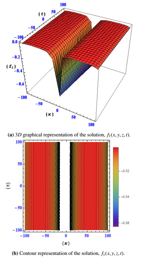
The objective of this work is to provide the method of getting the closed-form solitary wave solution of the fractional $ (3+1) $-generalized nonlinear wave equation that characterizes the behavior of liquids with gas bubbles. The same phenomena are evident in science, engineering, and even in the field of physics. This is done by employing the Riccati-Bernoulli sub-ode in a systematic manner as applied to the Bäcklund transformation in the study of this model. New soliton solutions, in the forms of soliton, are derived in the hyperbolic and trigonometric functions. The used software is the computational software Maple, which makes it possible to perform all the necessary calculations and the check of given solutions. The result of such calculations is graphical illustrations of the steady-state characteristics of the system and its dynamics concerning waves and the inter-relationships between the parameters. Moreover, the contour plots and the three-dimensional figures describe the essential features, helping readers understand the physical nature of the model introduced in this work.

| [1] | K. S. Miller, B. Ross, An introduction to the fractional calculus and fractional differential equations, New York: Wiley, 1993. |
| [2] | V. Daftardar-Gejji, Fractional calculus and fractional differential equations, Singapore: Springer, 2019. https://doi.org/10.1007/978-981-13-9227-6 |
| [3] |
S. Mukhtar, M. Sohaib, I. Ahmad, A numerical approach to solve volume-based batch crystallization model with fines dissolution unit, Processes, 7 (2019), 453. https://doi.org/10.3390/pr7070453 doi: 10.3390/pr7070453

|
| [4] |
M. Bouloudene, M. A. Alqudah, F. Jarad, Y. Adjabi, T. Abdeljawad, Nonlinear singular P-Laplacian boundary value problems in the frame of conformable derivative, Discret. Contin. Dyn. Syst. S, 14 (2021), 3497–3528. https://doi.org/10.3934/dcdss.2020442 doi: 10.3934/dcdss.2020442
|
| [5] |
T. Abdeljawad, On conformable fractional calculus, J. Comput. Appl. Math., 279 (2015), 57–66. https://doi.org/10.1016/j.cam.2014.10.016 doi: 10.1016/j.cam.2014.10.016
|
| [6] |
H. Yasmin, A. S. Alshehry, A. H. Ganie, A. M. Mahnashi, R. Shah, Perturbed Gerdjikov-Ivanov equation: Soliton solutions via Bäcklund transformation, Optik, 298 (2024), 171576. https://doi.org/10.1016/j.ijleo.2023.171576 doi: 10.1016/j.ijleo.2023.171576
|
| [7] |
A. Zafar, M. Raheel, A. M. Mahnashi, A. Bekir, M. R. Ali, A. S. Hendy, Exploring the new soliton solutions to the nonlinear M-fractional evolution equations in shallow water by three analytical techniques, Results Phys., 54 (2023), 107092. https://doi.org/10.1016/j.rinp.2023.107092 doi: 10.1016/j.rinp.2023.107092
|
| [8] |
W. Hamali, J. Manafian, M. Lakestani, A. M. Mahnashi, A. Bekir, Optical solitons of M-fractional nonlinear Schrödinger's complex hyperbolic model by generalized Kudryashov method, Opt. Quantum Electron., 56 (2024), 7. https://doi.org/10.1007/s11082-023-05602-1 doi: 10.1007/s11082-023-05602-1
|
| [9] |
I. Ahmad, H. Seno, An epidemic dynamics model with limited isolation capacity, Theory Biosci., 142 (2023), 259–273. https://doi.org/10.1007/s12064-023-00399-9 doi: 10.1007/s12064-023-00399-9
|
| [10] |
N. Iqbal, M. B. Riaz, M. Alesemi, T. S. Hassan, A. M. Mahnashi, A. Shafee, Reliable analysis for obtaining exact soliton solutions of (2+1)-dimensional Chaffee-Infante equation, AIMS Mathematics, 9 (2024), 16666–16686. https://doi.org/10.3934/math.2024808 doi: 10.3934/math.2024808
|
| [11] |
A. S. Alshehry, S. Mukhtar, A. M. Mahnashi, Analytical methods in fractional biological population modeling: Unveiling solitary wave solutions, AIMS Mathematics, 9 (2024), 15966–15987. https://doi.org/10.3934/math.2024773 doi: 10.3934/math.2024773
|
| [12] |
W. W. Mohammed, F. M. Al-Askar, C. Cesarano, M. El-Morshedy, Solitary wave solutions of the fractional-stochastic quantum Zakharov-Kuznetsov equation arises in quantum magneto plasma, Mathematics, 11 (2023), 488. https://doi.org/10.3390/math11020488 doi: 10.3390/math11020488
|
| [13] |
W. W. Mohammed, C. Cesarano, F. M. Al-Askar, Solutions to the (4+1)-dimensional time-fractional Fokas equation with M-truncated derivative, Mathematics, 11 (2023), 194. https://doi.org/10.3390/math11010194 doi: 10.3390/math11010194
|
| [14] |
W. W. Mohammed, F. M. Al-Askar, C. Cesarano, The analytical solutions of the stochastic mKdV equation via the mapping method, Mathematics, 10 (2022), 4212. https://doi.org/10.3390/math10224212 doi: 10.3390/math10224212
|
| [15] |
F. M. Al-Askar, C. Cesarano, W. W. Mohammed, The analytical solutions of stochastic-fractional Drinfeld-Sokolov-Wilson equations via (G'/G)-expansion method, Symmetry, 14 (2022), 2105. https://doi.org/10.3390/sym14102105 doi: 10.3390/sym14102105
|
| [16] | Y. Xie, I. Ahmad, T. I. Ikpe, E. F. Sofia, H., Seno, What influence could the acceptance of visitors cause on the epidemic dynamics of a reinfectious disease?: A mathematical model, Acta Biotheor., 72 (2024), 3. |
| [17] |
Y. Kai, Z. X. Yin, On the Gaussian traveling wave solution to a special kind of Schrödinger equation with logarithmic nonlinearity, Mod. Phys. Lett. B, 36 (2022), 2150543. https://doi.org/10.1142/S0217984921505436 doi: 10.1142/S0217984921505436
|
| [18] |
Y. Kai, S. Q. Chen, K. Zhang, Z. X. Yin, Exact solutions and dynamic properties of a nonlinear fourth-order time-fractional partial differential equation, Wave Random Complex, 2022. https://doi.org/10.1080/17455030.2022.2044541 doi: 10.1080/17455030.2022.2044541
|
| [19] |
C. Y. Zhu, M. Al-Dossari, S. Rezapour, B. Gunay, On the exact soliton solutions and different wave structures to the (2+1) dimensional Chaffee-Infante equation, Results Phys., 57 (2024), 107431. https://doi.org/10.1016/j.rinp.2024.107431 doi: 10.1016/j.rinp.2024.107431
|
| [20] |
Z. Wang, F. Parastesh, H. Natiq, J. Li, X. Xi, M. Mehrabbeik, Synchronization patterns in a network of diffusively delay-coupled memristive Chialvo neuron map, Phys. Lett. A, 514-515 (2024), 129607. https://doi.org/10.1016/j.physleta.2024.129607 doi: 10.1016/j.physleta.2024.129607
|
| [21] |
X. Xi, J. Li, Z. Wang, H. Tian, R. Yang, The effect of high-order interactions on the functional brain networks of boys with ADHD, Eur. Phys. J. Spec. Top., 233 (2024), 817–829. https://doi.org/10.1140/epjs/s11734-024-01161-y doi: 10.1140/epjs/s11734-024-01161-y
|
| [22] |
Z. Wang, M. Chen, X. Xi, H. Tian, R. Yang, Multi-chimera states in a higher order network of FitzHugh-Nagumo oscillators, Eur. Phys. J. Spec. Top., 233 (2024), 779–786. https://doi.org/10.1140/epjs/s11734-024-01143-0 doi: 10.1140/epjs/s11734-024-01143-0
|
| [23] |
T. A. A. Ali, Z. Xiao, H. Jiang, B. Li, A class of digital integrators based on trigonometric quadrature rules, IEEE Trans. Ind. Electron., 71 (2024), 6128–6138. https://doi.org/10.1109/TIE.2023.3290247 doi: 10.1109/TIE.2023.3290247
|
| [24] |
G. Shen, J. Manafian, D. T. N. Huy, K. S. Nisar, M. Abotaleb, N. D. Trung, Abundant soliton wave solutions and the linear superposition principle for generalized (3+1)-D nonlinear wave equation in liquid with gas bubbles by bilinear analysis, Results Phys., 32 (2022), 105066. https://doi.org/10.1016/j.rinp.2021.105066 doi: 10.1016/j.rinp.2021.105066
|
| [25] |
M. Wang, B. Tian, Y. Sun, Z. Zhang, Lump, mixed lump-stripe and rogue wave-stripe solutions of a (3+1)-dimensional nonlinear wave equation for a liquid with gas bubbles, Comput. Math. Appl., 79 (2020), 576–587. https://doi.org/10.1016/j.camwa.2019.07.006 doi: 10.1016/j.camwa.2019.07.006
|
| [26] |
Y. R. Guo, A. H. Chen, Hybrid exact solutions of the (3+1)-dimensional variable-coefficient nonlinear wave equation in liquid with gas bubbles, Results Phys., 23 (2021), 103926. https://doi.org/10.1016/j.rinp.2021.103926 doi: 10.1016/j.rinp.2021.103926
|
| [27] |
X. J. Zhou, O. A. Ilhan, F. Y. Zhou, S. Sutarto, J. Manafian, M. Abotaleb, Lump and interaction solutions to the (3+1)-dimensional variable-coefficient nonlinear wave equation with multidimensional binary Bell polynomials, J. Funct. Space, 2021 (2021), 4550582. https://doi.org/10.1155/2021/4550582 doi: 10.1155/2021/4550582
|
| [28] |
Y. H. Zhao, T. Mathanaranjan, H. Rezazadeh, L. Akinyemi, M. Inc, New solitary wave solutions and stability analysis for the generalized (3+1)-dimensional nonlinear wave equation in liquid with gas bubbles, Results Phys., 43 (2022), 106083. https://doi.org/10.1016/j.rinp.2022.106083 doi: 10.1016/j.rinp.2022.106083
|
| [29] | A. Akbulut, A. H. Arnous, M. S. Hashemi, M. Mirzazadeh, Solitary waves for the generalized nonlinear wave equation in (3+1) dimensions with gas bubbles using Nucci's reduction, enhanced and modified Kudryashov algorithms, J. Ocean. Eng. Sci., 2022, In press. https://doi.org/10.1016/j.joes.2022.07.002 |
| [30] | E. M. E. Zayed, K. A. E. Alurrfi, The modified extended tanh-function method and its applications to the generalized KdV-mKdV equation with any-order nonlinear terms, Int. J. Environ. Eng. Sci. Tech. Res., 1 (2013), 165–170. |
| [31] |
S. Alshammari, M. M. Al-Sawalha, R. Shah, Approximate analytical methods for a fractional-order nonlinear system of Jaulent-Miodek equation with energy-dependent Schrodinger potential, Fractal Fract., 7 (2023), 140. https://doi.org/10.3390/fractalfract7020140 doi: 10.3390/fractalfract7020140
|
| [32] |
A. A. Alderremy, R. Shah, N. Iqbal, S. Aly, K. Nonlaopon, Fractional series solution construction for nonlinear fractional reaction-diffusion Brusselator model utilizing Laplace residual power series, Symmetry, 14 (2022), 1944. https://doi.org/10.3390/sym14091944 doi: 10.3390/sym14091944
|
| [33] |
M. M. Al-Sawalha, R. Shah, A. Khan, O. Y. Ababneh, T. Botmart, Fractional view analysis of Kersten-Krasil-shchik coupled KdV-mKdV systems with non-singular kernel derivatives, AIMS Mathematics, 7 (2022), 18334–18359. https://doi.org/10.3934/math.20221010 doi: 10.3934/math.20221010
|
| [34] |
E. M. Elsayed, R. Shah, K. Nonlaopon, The analysis of the fractional-order Navier-Stokes equations by a novel approach, J. Funct. Space, 2022 (2022), 8979447. https://doi.org/10.1155/2022/8979447 doi: 10.1155/2022/8979447
|
| [35] |
M. Alqhtani, K. M. Saad, R. Shah, W. Weera, W. M. Hamanah, Analysis of the fractional-order local Poisson equation in fractal porous media, Symmetry, 14 (2022), 1323. https://doi.org/10.3390/sym14071323 doi: 10.3390/sym14071323
|
| [36] |
M. Naeem, H. Rezazadeh, A. A. Khammash, R. Shah, S. Zaland, Analysis of the fuzzy fractional-order solitary wave solutions for the KdV equation in the sense of Caputo-Fabrizio derivative, J. Math., 2022 (2022), 3688916. https://doi.org/10.1155/2022/3688916 doi: 10.1155/2022/3688916
|
| [37] |
M. A. E. Abdelrahman, M. A. Sohaly, Solitary waves for the modified Korteweg-de Vries equation in deterministic case and random case, J. Phys. Math., 8 (2017), 1000214. https://doi.org/10.4172/2090-0902.1000214 doi: 10.4172/2090-0902.1000214
|
| [38] |
M. A. E. Abdelrahman, M. A. Sohaly, Solitary waves for the nonlinear Schrödinger problem with the probability distribution function in the stochastic input case, Eur. Phys. J. Plus, 132 (2017), 339. https://doi.org/10.1140/epjp/i2017-11607-5 doi: 10.1140/epjp/i2017-11607-5
|
| [39] |
X. F. Yang, Z. C. Deng, Y. Wei, A Riccati-Bernoulli sub-ODE method for nonlinear partial differential equations and its application, Adv. Differ. Equ., 2015 (2015), 117. https://doi.org/10.1186/s13662-015-0452-4 doi: 10.1186/s13662-015-0452-4
|
| [40] |
Y. Jawarneh, H. Yasmin, A. H. Ganie, M. M. Al-Sawalha, A. Ali, Unification of adomian decomposition method and zz transformation for exploring the dynamics of fractional kersten-krasil'shchik coupled kdv-mkdv systems, AIMS Mathematics, 9 (2024), 371–390. https://doi.org/10.3934/math.2024021 doi: 10.3934/math.2024021
|
| [41] |
S. Bibi, S. T. Mohyud-Din, R. Ullah, N. Ahmed, U. Khan, Exact solutions for STO and (3+1)-dimensional KdV-ZK equations using $G'/G$-expansion method, Results Phys., 7 (2017), 4434–4439. https://doi.org/10.1016/j.rinp.2017.11.009 doi: 10.1016/j.rinp.2017.11.009
|


Figures(4) / Tables(1)

Musawa Yahya Almusawa, Hassan Almusawa. Dark and bright soliton phenomena of the generalized time-space fractional equation with gas bubbles[J]. AIMS Mathematics, 2024, 9(11): 30043-30058. doi: 10.3934/math.20241451


 DownLoad: