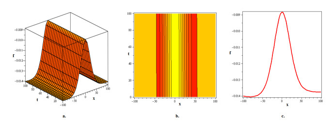
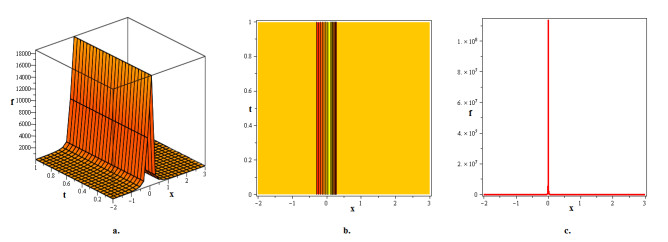
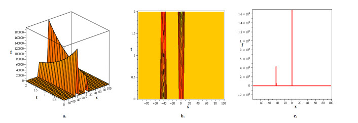
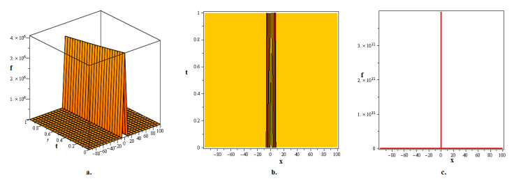
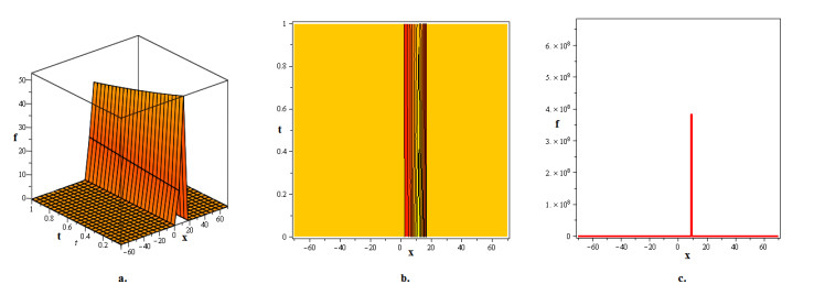
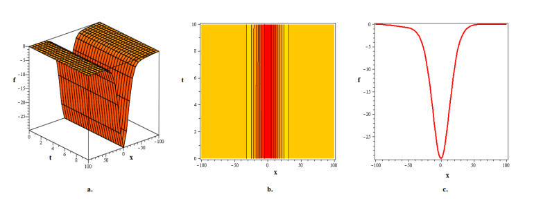
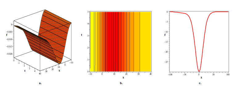
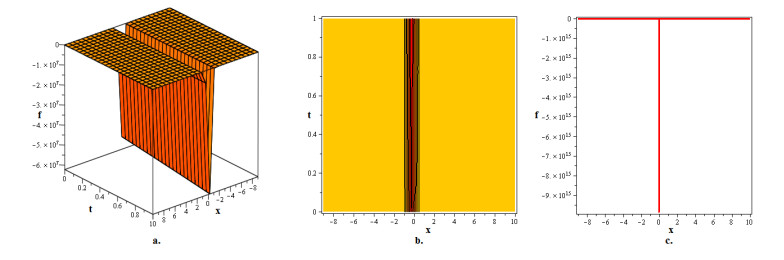
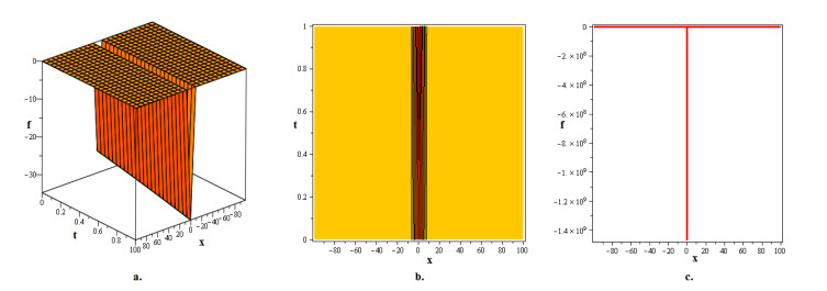
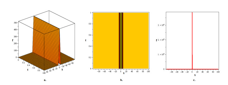
This study explored and examined soliton solutions for the Quintic Benney-Lin equation (QBLE), which describes the dynamic of liquid films, using the Riccati modified extended simple equation method (RMESEM). The proposed approach, which is designed for nonlinear partial differential equations (NPDEs), effectively generates a large number of soliton solutions for the given QBLE, which basically captures the fundamental dynamics of the system. The rational, hyperbolic, rational-hyperbolic, trigonometric, and exponential forms of the scientifically specified soliton solutions are the main determinants of the hump solitons. We used 2D, 3D, and contour visualizations to offer accurate representations of the researched soliton phenomena associated with these solutions. These representations revealed the existence of dark and bright hump solitons in the framework of the QBLE and offer a thorough way to examine the model's behavioral characteristics in the liquid film by analyzing the QBLE model's soliton dynamics. Moreover, applying the suggested approach advances our knowledge of the unique features of the other similar NPDEs and the underlying dynamics.
Citation: Waleed Hamali, Hamad Zogan, Abdulhadi A. Altherwi. Dark and bright hump solitons in the realm of the quintic Benney-Lin equation governing a liquid film[J]. AIMS Mathematics, 2024, 9(10): 29167-29196. doi: 10.3934/math.20241414
This study explored and examined soliton solutions for the Quintic Benney-Lin equation (QBLE), which describes the dynamic of liquid films, using the Riccati modified extended simple equation method (RMESEM). The proposed approach, which is designed for nonlinear partial differential equations (NPDEs), effectively generates a large number of soliton solutions for the given QBLE, which basically captures the fundamental dynamics of the system. The rational, hyperbolic, rational-hyperbolic, trigonometric, and exponential forms of the scientifically specified soliton solutions are the main determinants of the hump solitons. We used 2D, 3D, and contour visualizations to offer accurate representations of the researched soliton phenomena associated with these solutions. These representations revealed the existence of dark and bright hump solitons in the framework of the QBLE and offer a thorough way to examine the model's behavioral characteristics in the liquid film by analyzing the QBLE model's soliton dynamics. Moreover, applying the suggested approach advances our knowledge of the unique features of the other similar NPDEs and the underlying dynamics.

| [1] |
R. Ali, Z. Zhang, H. Ahmad, Exploring soliton solutions in nonlinear spatiotemporal fractional quantum mechanics equations: an analytical study, Opt. Quant. Electron., 56 (2024), 838. https://doi.org/10.1007/s11082-024-06370-2 doi: 10.1007/s11082-024-06370-2

|
| [2] |
Y. Kai, Z. Yin, On the Gaussian traveling wave solution to a special kind of Schröinger equation with logarithmic nonlinearity, Mod. Phys. Lett. B, 36 (2021), 2150543. https://doi.org/10.1142/S0217984921505436 doi: 10.1142/S0217984921505436
|
| [3] | Y. Kai, S. Chen, K. Zhang, Z. Yin, Exact solutions and dynamic properties of a nonlinear fourth-order time-fractional partial differential equation, Waves Random Complex Media, 2022. https://doi.org/10.1080/17455030.2022.2044541 |
| [4] |
Y., Kai, Z. Yin, Linear structure and soliton molecules of Sharma-Tasso-Olver-Burgers equation, Phys. Lett. A, 452 (2022), 128430. https://doi.org/10.1016/j.physleta.2022.128430 doi: 10.1016/j.physleta.2022.128430
|
| [5] | Q. Wu, N. Chen, M. Yao, Y. Niu, C. Wang, Nonlinear dynamic analysis of FG fluid conveying micropipes with initial imperfections, Int. J. Struct. Stab. Dyn., 2024. https://doi.org/10.1142/S0219455425500178 |
| [6] |
L. Liu, S. Zhang, L. Zhang, G. Pan, J. Yu, Multi-UUV maneuvering counter-game for dynamic target scenario based on fractional-order recurrent neural network, IEEE Trans. Cybern., 53 (2023), 4015–4028. https://doi.org/10.1109/TCYB.2022.3225106 doi: 10.1109/TCYB.2022.3225106
|
| [7] |
A. Gaber, H. Ahmad, Solitary wave solutions for space-time fractional coupled integrable dispersionless system via generalized Kudryashov method, Facta Univ. Ser.: Math. Inf., 2021 (2021), 1439–1449. https://doi.org/10.22190/FUMI2005439G doi: 10.22190/FUMI2005439G
|
| [8] |
H. Yasmin, N. H. Aljahdaly, A. M. Saeed, R. Shah, Probing families of optical soliton solutions in fractional perturbed Radhakrishnan-Kundu-Lakshmanan model with improved versions of extended direct algebraic method, Fractal Fract., 7 (2023), 512. https://doi.org/10.3390/fractalfract7070512 doi: 10.3390/fractalfract7070512
|
| [9] |
M. Younis, M. Iftikhar, Computational examples of a class of fractional order nonlinear evolution equations using modified extended direct algebraic method, J. Comput. Methods Sci. Eng., 15 (2015), 359–365. https://doi.org/10.3233/JCM-150548 doi: 10.3233/JCM-150548
|
| [10] |
Y. Tian, J. Liu, A modified exp-function method for fractional partial differential equations, Therm. Sci., 25 (2021), 1237–1241. https://doi.org/10.2298/TSCI200428017T doi: 10.2298/TSCI200428017T
|
| [11] |
M. M. A. Khater, Computational simulations of propagation of a tsunami wave across the ocean, Chaos Soliton. Fract., 174 (2023), 113806. https://doi.org/10.1016/j.chaos.2023.113806 doi: 10.1016/j.chaos.2023.113806
|
| [12] |
W. Alhejaili, E. Az-Zo'bi, R. Shah, S. A. El-Tantawy, On the analytical soliton approximations to fractional forced Korteweg-de Vries equation arising in fluids and Plasmas using two novel techniques, Commun. Theor. Phys., 76 (2024), 085001. https://doi.org/10.1088/1572-9494/ad53bc doi: 10.1088/1572-9494/ad53bc
|
| [13] |
M. A. Bayrak, A. Demir, A new approach for space-time fractional partial differential equations by residual power series method, Appl. Math. Comput., 336 (2018), 215–230. https://doi.org/10.1016/j.amc.2018.04.032 doi: 10.1016/j.amc.2018.04.032
|
| [14] |
O. A. Arqub, Numerical simulation of time-fractional partial differential equations arising in fluid flows via reproducing Kernel method, Int. J. Numer. Methods Heat Fluid Flow, 30 (2020), 4711–4733. https://doi.org/10.1108/HFF-10-2017-0394 doi: 10.1108/HFF-10-2017-0394
|
| [15] | M. Kaplan, A. Bekir, A. Akbulut, E. Aksoy, The modified simple equation method for nonlinear fractional differential equations, Rom. J. Phys., 60 (2015), 1374–1383. |
| [16] |
S. Akcagil, T. Aydemir, A new application of the unified method, New Trends Math. Sci., 6 (2018), 185–199. https://doi.org/10.20852/ntmsci.2018.261 doi: 10.20852/ntmsci.2018.261
|
| [17] |
M. Eslami, B. Fathi Vajargah, M. Mirzazadeh, A. Biswas, Application of first integral method to fractional partial differential equations, Indian J. Phys., 88 (2014), 177–184. https://doi.org/10.1007/s12648-013-0401-6 doi: 10.1007/s12648-013-0401-6
|
| [18] |
N. M. Rasheed, M. O. Al-Amr, E. A. Az-Zobi, M. A. Tashtoush, L. Akinyemi, Stable optical solitons for the Higher-order Non-Kerr NLSE via the modified simple equation method, Mathematics, 9 (2021), 1986. https://doi.org/10.3390/math9161986 doi: 10.3390/math9161986
|
| [19] |
P. G. Estévez, E. Conde, P. R. Gordoa, Unified approach to Miura, Bäcklund and Darboux transformations for nonlinear partial differential equations, J. Nonlinear Math. Phys., 5 (1998), 82–114. https://doi.org/10.2991/jnmp.1998.5.1.8 doi: 10.2991/jnmp.1998.5.1.8
|
| [20] |
N. K. Vitanov, Z. I. Dimitrova, Simple equations method (SEsM) and its particular cases: Hirota method, AIP Conf. Proc., 2321 (2021), 030036. https://doi.org/10.1063/5.0040410 doi: 10.1063/5.0040410
|
| [21] |
Y. Xiao, S. Barak, M. Hleili, K. Shah, Exploring the dynamical behaviour of optical solitons in integrable kairat-II and kairat-X equations, Phys. Scr., 99 (2024), 095261. https://doi.org/10.1088/1402-4896/ad6e34 doi: 10.1088/1402-4896/ad6e34
|
| [22] |
S. Alshammari, M. M. Al-Sawalha, R. Shah, Approximate analytical methods for a fractional-order nonlinear system of Jaulent-Miodek equation with energy-dependent Schrödinger potential, Fractal Fract., 7 (2023), 140. https://doi.org/10.3390/fractalfract7020140 doi: 10.3390/fractalfract7020140
|
| [23] |
A. A. Alderremy, R. Shah, N. Iqbal, S. Aly, K. Nonlaopon, Fractional series solution construction for nonlinear fractional reaction-diffusion Brusselator model utilizing Laplace residual power series, Symmetry, 14 (2022), 1944. https://doi.org/10.3390/sym14091944 doi: 10.3390/sym14091944
|
| [24] |
A. H. Arnous, A. Biswas, A. H. Kara, Y. Yıldırım, L. Moraru, C. Iticescu, et al., Optical solitons and conservation laws for the concatenation model with spatio-temporal dispersion (internet traffic regulation), J. Eur. Opt. Society-Rapid Publ., 19 (2023), 35. https://doi.org/10.1051/jeos/2023031 doi: 10.1051/jeos/2023031
|
| [25] |
M. M. Al-Sawalha, R. Shah, A. Khan, O. Y. Ababneh, T. Botmart, Fractional view analysis of Kersten-Krasil'shchik coupled KdV-mKdV systems with non-singular kernel derivatives, AIMS Math., 7 (2022), 18334–18359. https://doi.org/10.3934/math.20221010 doi: 10.3934/math.20221010
|
| [26] |
H. Yasmin, A. S. Alshehry, A. H. Ganie, A. M. Mahnashi, R. Shah, Perturbed Gerdjikov-Ivanov equation: soliton solutions via Backlund transformation, Optik, 298 (2024), 171576. https://doi.org/10.1016/j.ijleo.2023.171576 doi: 10.1016/j.ijleo.2023.171576
|
| [27] |
E. M. Elsayed, R. Shah, K. Nonlaopon, The analysis of the fractional-order Navier-Stokes equations by a novel approach, J. Funct. Spaces, 2022 (2022), 8979447. https://doi.org/10.1155/2022/8979447 doi: 10.1155/2022/8979447
|
| [28] | R. Ali, D. Kumar, A. Akgul, A. Altalbe, On the periodic soliton solutions for fractional Schrödinger equations, Fractals, 2024. https://doi.org/10.1142/S0218348X24400334 |
| [29] |
M. Alqhtani, K. M. Saad, W. M. Hamanah, Discovering novel soliton solutions for $(3+1)$-modified fractional Zakharov-Kuznetsov equation in electrical engineering through an analytical approach, Opt. Quant. Electron., 55 (2023), 1149. https://doi.org/10.1007/s11082-023-05407-2 doi: 10.1007/s11082-023-05407-2
|
| [30] |
M. Alqhtani, K. M. Saad, R. Shah, W. Weera, W. M. Hamanah, Analysis of the fractional-order local Poisson equation in fractal porous media, Symmetry, 14 (2022), 1323. https://doi.org/10.3390/sym14071323 doi: 10.3390/sym14071323
|
| [31] |
M. Bilal, J. Iqbal, R. Ali, F. A. Awwad, E. A. A. Ismail, Establishing breather and $N$-soliton solutions for conformable Klein-Gordon equation, Open Phys., 22 (2024), 20240044 https://doi.org/10.1515/phys-2024-0044 doi: 10.1515/phys-2024-0044
|
| [32] |
R. Ali, Z. Zhang, H. Ahmad, M. M. Alam, The analytical study of soliton dynamics in fractional coupled Higgs system using the generalized Khater method, Opt. Quant. Electron., 56 (2024), 1067. https://doi.org/10.1007/s11082-024-06924-4 doi: 10.1007/s11082-024-06924-4
|
| [33] |
C. Zhu, M. Al-Dossari, S. Rezapour, B. Gunay, On the exact soliton solutions and different wave structures to the $(2+1)$ dimensional Chaffee-Infante equation, Results Phys., 57 (2024), 107431. https://doi.org/10.1016/j.rinp.2024.107431 doi: 10.1016/j.rinp.2024.107431
|
| [34] |
T. A. A. Ali, Z. Xiao, H. Jiang, B. Li, A class of digital integrators based on trigonometric quadrature rules, IEEE Trans. Ind. Electron., 71 (2024), 6128–6138. https://doi.org/10.1109/TIE.2023.3290247 doi: 10.1109/TIE.2023.3290247
|
| [35] |
M. M. A. Khater, Advanced computational techniques for solving the modified KdV-KP equation and modeling nonlinear waves, Opt. Quant. Electron., 56 (2024), 6. https://doi.org/10.1007/s11082-023-05581-3 doi: 10.1007/s11082-023-05581-3
|
| [36] |
M. M. A. Khater, Waves in motion: unraveling nonlinear behavior through the Gilson-Pickering equation, Eur. Phys. J. Plus, 138 (2023), 1138. https://doi.org/10.1140/epjp/s13360-023-04774-9 doi: 10.1140/epjp/s13360-023-04774-9
|
| [37] |
M. M. A. Khater, Analyzing pulse behavior in optical fiber: novel solitary wave solutions of the perturbed Chen-Lee-Liu equation, Mod. Phys. Lett. B, 37 (2023), 2350177. https://doi.org/10.1142/S0217984923501774 doi: 10.1142/S0217984923501774
|
| [38] |
M. M. A. Khater, Exploring the rich solution landscape of the generalized Kawahara equation: insights from analytical techniques, Eur. Phys. J. Plus, 139 (2024), 184. https://doi.org/10.1140/epjp/s13360-024-04971-0 doi: 10.1140/epjp/s13360-024-04971-0
|
| [39] |
M. M. A. Khater, Wave propagation and evolution in a $(1+1)$-dimensional spatial-temporal domain: a comprehensive study, Mod. Phys. Lett. B, 38 (2024), 2350235. https://doi.org/10.1142/S0217984923502354 doi: 10.1142/S0217984923502354
|
| [40] |
M. M. A. Khater, Dynamics of nonlinear time fractional equations in shallow water waves, Int. J. Theor. Phys., 63 (2024), 92. https://doi.org/10.1007/s10773-024-05634-7 doi: 10.1007/s10773-024-05634-7
|
| [41] |
M. M. A. Khater, Computational method for obtaining solitary wave solutions of the $(2+ 1)$-dimensional AKNS equation and their physical significance, Mod. Phys. Lett. B, 38 (2024), 2350252. https://doi.org/10.1142/S0217984923502524 doi: 10.1142/S0217984923502524
|
| [42] |
S. P. Lin, Finite amplitude side-band stability of a viscous film, J. Fluid Mech., 63 (1974), 417–429. https://doi.org/10.1017/S0022112074001704 doi: 10.1017/S0022112074001704
|
| [43] | D. Benney, Long waves on liquid films, J. Math. Phys., 45 (1966), 150–155. https://doi.org/10.1002/sapm1966451150 |
| [44] |
W. Gao, P. Veeresha, D. G. Prakasha, H. M. Baskonus, New numerical simulation for fractional Benney-Lin equation arising in falling film problems using two novel techniques, Numer. Methods Partial Differ. Equ., 37 (2021), 210–243. https://doi.org/10.1002/num.22526 doi: 10.1002/num.22526
|
| [45] |
N. G. Berloff, L. N. Howard, Solitary and periodic solutions of nonlinear nonintegrable equations, Stud. Appl. Math., 99 (1997), 1–24. https://doi.org/10.1111/1467-9590.00054 doi: 10.1111/1467-9590.00054
|
| [46] |
H. A. Biagioni, F. Linares, On the Benney-Lin and Kawahara equations, J. Math. Anal. Appl., 211 (1997), 131–152. https://doi.org/10.1006/jmaa.1997.5438 doi: 10.1006/jmaa.1997.5438
|
| [47] |
S. B. Cui, D. G. Deng, S. P. Tao, Global existence of solutions for the Cauchy problem of the Kawahara equation with $L^2$ initial data, Acta Math. Sinica, 22 (2006), 1457–1466. https://doi.org/10.1007/s10114-005-0710-6 doi: 10.1007/s10114-005-0710-6
|
| [48] |
H. Tariq, G. Akram, Residual power series method for solving time-space-fractional Benney-Lin equation arising in falling film problems, J. Appl. Math. Comput., 55 (2017), 683–708. https://doi.org/10.1007/s12190-016-1056-1 doi: 10.1007/s12190-016-1056-1
|
| [49] |
Y. X. Xie, New explicit and exact solutions of the Benney-Kawahara-Lin equation, Chin. Phys. B, 18 (2009), 4094. https://doi.org/10.1088/1674-1056/18/10/005 doi: 10.1088/1674-1056/18/10/005
|
| [50] |
N. Mshary, Exploration of nonlinear traveling wave phenomena in quintic conformable Benney-Lin equation within a liquid film, AIMS Math., 9 (2024), 11051–11075. https://doi.org/10.3934/math.2024542 doi: 10.3934/math.2024542
|
| [51] |
P. K. Gupta, Approximate analytical solutions of fractional Benney-Lin equation by reduced differential transform method and the homotopy perturbation method, Comput. Math. Appl., 61 (2011), 2829–2842. https://doi.org/10.1016/j.camwa.2011.03.057 doi: 10.1016/j.camwa.2011.03.057
|
| [52] |
Z. Navickas, R. Marcinkevicius, I. Telksniene, T. Telksnys, M. Ragulskis, Structural stability of the hepatitis $C$ model with the proliferation of infected and uninfected hepatocytes, Math. Comput. Model. Dyn. Syst., 30 (2024), 51–72. https://doi.org/10.1080/13873954.2024.2304808 doi: 10.1080/13873954.2024.2304808
|
| [53] |
I. Ullah, K. Shah, S. Barak, T. Abdeljawad, Pioneering the plethora of soliton for the $(3+ 1)$-dimensional fractional heisenberg ferromagnetic spin chain equation, Phys. Scr., 99 (2024), 095229. https://doi.org/10.1088/1402-4896/ad6ae6 doi: 10.1088/1402-4896/ad6ae6
|
| [54] |
E. Fan, Extended tanh-function method and its applications to nonlinear equations, Phys. Lett. A, 277 (2000), 212–218. https://doi.org/10.1016/S0375-9601(00)00725-8 doi: 10.1016/S0375-9601(00)00725-8
|
| [55] |
D. Wang, H. Q. Zhang, Further improved $F$-expansion method and new exact solutions of Konopelchenko-Dubrovsky equation, Chaos Soliton. Fract., 25 (2005), 601–610. https://doi.org/10.1016/j.chaos.2004.11.026 doi: 10.1016/j.chaos.2004.11.026
|
Figures(10)

Waleed Hamali, Hamad Zogan, Abdulhadi A. Altherwi. Dark and bright hump solitons in the realm of the quintic Benney-Lin equation governing a liquid film[J]. AIMS Mathematics, 2024, 9(10): 29167-29196. doi: 10.3934/math.20241414


 DownLoad: