


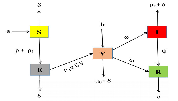
Figure 1.
The flow chart illustrates the newly developed model.
Outdoor, real-time, and accurate detection of insulator defect locations can effectively avoid the occurrence of power grid security accidents. This paper proposes an improved GhostNet-YOLOv5s algorithm based on GhostNet and YOLOv5 models. First, the backbone feature extraction network of YOLOv5 was reconstructed with the lightweight GhostNet module to reduce the number of parameters and floating point operations of the model, so as to achieve the purpose of being lightweight. Then, a 160 × 160 feature layer was added to the YOLOv5 network to extract more feature information of small targets and fuzzy targets. In addition, the introduction of lightweight GSConv convolution in the neck network further reduced the computing cost of the entire network. Finally, Focal-EIoU was introduced to optimize the CIoU bounding box regression loss function in the original algorithm to improve the convergence speed and target location accuracy of the model. The experimental results show that the parameter number, computation amount, and model size of the GhostNet-YOLOv5s model are reduced by 40%, 25%, and 36%, respectively, compared with the unimproved YOLOv5s model. The proposed method not only ensures the precision of insulator defect detection, but also greatly decreases the complexity of the model. Therefore, the GhostNet-YOLOv5s algorithm can meet the requirements of real-time detection in complex outdoor environments.
Citation: Jianjun Huang, Xuhong Huang, Ronghao Kang, Zhihong Chen, Junhan Peng. Improved insulator location and defect detection method based on GhostNet and YOLOv5s networks[J]. Electronic Research Archive, 2024, 32(9): 5249-5267. doi: 10.3934/era.2024242
| [1] | Xiao Xu, Hong Liao, Xu Yang . An automatic density peaks clustering based on a density-distance clustering index. AIMS Mathematics, 2023, 8(12): 28926-28950. doi: 10.3934/math.20231482 |
| [2] | Fatimah Alshahrani, Wahiba Bouabsa, Ibrahim M. Almanjahie, Mohammed Kadi Attouch . kNN local linear estimation of the conditional density and mode for functional spatial high dimensional data. AIMS Mathematics, 2023, 8(7): 15844-15875. doi: 10.3934/math.2023809 |
| [3] | Shabbar Naqvi, Muhammad Salman, Muhammad Ehtisham, Muhammad Fazil, Masood Ur Rehman . On the neighbor-distinguishing in generalized Petersen graphs. AIMS Mathematics, 2021, 6(12): 13734-13745. doi: 10.3934/math.2021797 |
| [4] | Yuming Chen, Jie Gao, Luan Teng . Distributed adaptive event-triggered control for general linear singular multi-agent systems. AIMS Mathematics, 2023, 8(7): 15536-15552. doi: 10.3934/math.2023792 |
| [5] | Luca Bisconti, Paolo Maria Mariano . Global existence and regularity for the dynamics of viscous oriented fluids. AIMS Mathematics, 2020, 5(1): 79-95. doi: 10.3934/math.2020006 |
| [6] | Hsin-Lun Li . Leader–follower dynamics: stability and consensus in a socially structured population. AIMS Mathematics, 2025, 10(2): 3652-3671. doi: 10.3934/math.2025169 |
| [7] | Hongjie Li . Event-triggered bipartite consensus of multi-agent systems in signed networks. AIMS Mathematics, 2022, 7(4): 5499-5526. doi: 10.3934/math.2022305 |
| [8] | Neelakandan Subramani, Abbas Mardani, Prakash Mohan, Arunodaya Raj Mishra, Ezhumalai P . A fuzzy logic and DEEC protocol-based clustering routing method for wireless sensor networks. AIMS Mathematics, 2023, 8(4): 8310-8331. doi: 10.3934/math.2023419 |
| [9] | Yinwan Cheng, Chao Yang, Bing Yao, Yaqin Luo . Neighbor full sum distinguishing total coloring of Halin graphs. AIMS Mathematics, 2022, 7(4): 6959-6970. doi: 10.3934/math.2022386 |
| [10] | Jin Cai, Shuangliang Tian, Lizhen Peng . On star and acyclic coloring of generalized lexicographic product of graphs. AIMS Mathematics, 2022, 7(8): 14270-14281. doi: 10.3934/math.2022786 |
Outdoor, real-time, and accurate detection of insulator defect locations can effectively avoid the occurrence of power grid security accidents. This paper proposes an improved GhostNet-YOLOv5s algorithm based on GhostNet and YOLOv5 models. First, the backbone feature extraction network of YOLOv5 was reconstructed with the lightweight GhostNet module to reduce the number of parameters and floating point operations of the model, so as to achieve the purpose of being lightweight. Then, a 160 × 160 feature layer was added to the YOLOv5 network to extract more feature information of small targets and fuzzy targets. In addition, the introduction of lightweight GSConv convolution in the neck network further reduced the computing cost of the entire network. Finally, Focal-EIoU was introduced to optimize the CIoU bounding box regression loss function in the original algorithm to improve the convergence speed and target location accuracy of the model. The experimental results show that the parameter number, computation amount, and model size of the GhostNet-YOLOv5s model are reduced by 40%, 25%, and 36%, respectively, compared with the unimproved YOLOv5s model. The proposed method not only ensures the precision of insulator defect detection, but also greatly decreases the complexity of the model. Therefore, the GhostNet-YOLOv5s algorithm can meet the requirements of real-time detection in complex outdoor environments.
Mathematics was initially utilized in biology in the 13th century by Fibonacci, who developed the famed Fibonacci series to explain an increasing population. Daniel Bernoulli utilized mathematics to describe the impact on tiny shapes. Johannes Reinke coined the phrase "bio maths" in 1901. Biomathematics involves the theoretical examination of mathematical models to understand the principles governing the formation and functioning of biological systems.
Mathematical models are utilized to investigate specific questions related to the studied disease. For example, epidemiological models are important for predicting how infectious diseases spread, and help to control them by identifying important factors in the community. In this case, we want to analyze a particular model to understand how the COVID-19 virus behaves. This virus appeared in late 2019, and continues to be a global challenge. To gain a deeper insight into the underlying physical processes, we delve into the realm of fractional calculus. Previous literature has introduced various operators through the framework of fractional calculus [1,2]. In the field of Cη-Calculus, Golmankhaneh et al. [3] provided an explanation of the Sumudu transform and Laplace transform. Additionally, in 2019, Goyal [4] proposed a fractional model that demonstrated the potential to manage the Lassa hemorrhagic fever disease.
Advancements in technology have led to significant progress in the field of epidemiology, enabling the examination of various infectious diseases for treatment, control, and cure [5]. It is essential to underscore that mathematical biology plays a pivotal role in investigating numerous diseases. Significant strides have been taken in the mathematical modeling of infectious diseases in recent decades, as evidenced by various studies [6,7]. Over the last thirty years, mathematical modeling has gained prominence in research, making substantial contributions to the development of effective public health strategies for disease control [8,9]. Mathematical models serve as invaluable tools for analyzing spatiotemporal patterns and the dynamic behavior of infections. Acknowledging their significance, researchers have approached the study of COVID-19 from diverse perspectives in the last three years [10,11].
Various methodologies have been employed by researchers in this field to devise successful techniques for managing this condition, with recent studies offering additional insights [12,13]. For example, a recent investigation utilized a mathematical model to evaluate the impacts of immunization in nursing homes [14]. Furthermore, researchers have explored mathematical modeling and effective intervention strategies for controlling the COVID-19 outbreak [15]. Additionally, some studies have delved into COVID-19 mathematical models using stochastic differential equations and environmental white noise [16].
In 2019, China experienced a notable outbreak of the coronavirus disease 2019 (COVID-19), prompting concerns about its potential to escalate into a worldwide pandemic [17]. Researchers from China, particularly Zhao et al., made significant contributions in addressing the challenges posed by COVID-19. This disease is attributed to the severe acute respiratory syndrome coronavirus 2 (SARS-CoV-2), a viral infection. The initial verified case was documented in Wuhan, China, in December 2019 [18]. The infection rapidly spread worldwide, leading to the declaration of a COVID-19 pandemic.
Transmission occurs through various means, including respiratory droplets from coughing, sneezing, close contact, and touching contaminated surfaces. Key preventive measures include consistent mask usage, frequent hand washing, and maintaining safe interpersonal distances [19]. Effective interventions and real-time data play a crucial role in managing the coronavirus outbreak [20]. Prior studies have employed real-time analysis to comprehend the transmission of the virus among individuals, the severity of the disease, and the early stages of the pathogen, particularly in the initial week of the outbreak [21].
In December 2019, an outbreak of pneumonia cases was reported in Wuhan, initially with unidentified origins. Some cases were associated with exposure to wet markets and seafood. Chinese health authorities, in collaboration with the Chinese Center for Disease Control and Prevention (China CDC), initiated an investigation into the cause and spread of the disease on December 31, 2019 [22]. We conducted an analysis of temporal changes in the outbreak by examining the time interval between hospital admission dates and fatalities. Clinical studies on COVID-19 have indicated that symptoms typically manifest around 7 days after the onset of illness [23]. It is important to consider the duration between hospitalization and death in order to accurately assess the risk of mortality [24]. The information regarding the incubation period of COVID-19 and epidemiological data was sourced from publicly available records of confirmed cases [25].
An established method for the fractional-order model is elaborated upon in [26]. Recent contributions include various fractional models related to COVID-19, such as the analysis by Atangana and Khan focusing on the pandemic's impact on China [27]. Additionally, the COVID-19 model's dynamical aspects were explored using fuzzy Caputo and ABC derivatives, as demonstrated in [28]. A similar type of approach using fractional operator techniques are given in [29,30,31]. Different author's have investigated the transmission of different infectious disease like COVID-19 with symptomatic and asymptomatic effects in the community by using the fractal-fractional definition [32,33].
In light of the aforementioned significance, we aim is to address fundamental issues by concentrating on the distinctive challenges posed by the dynamics of COVID-19. To achieve this, we employ a model tailored to accurately capture the characteristics of COVID-19 dynamics and account for the limitations in our response to the pandemic. Initially, we examine the epidemic dynamics within a specific community characterized by a unique social pattern. For this analysis, we adopt a conventional SEIR design that accommodates prolonged incubation periods.
Here, the previous model is given in [34] as follows:
| dSdt=a−ρ1SI1+γI−(δ+ρ)S,dEdt=ρS−δE−ρ2αEI,dIdt=ρ1SI1+γI+ρ2αEI−(δ+μ0+ω−b)I,dRdt=ωI−δR. | (1.1) |
Initial conditions corresponds to the aforementioned system:
| S0(t)=S0,E0(t)=E0,I0(t)=I0,R0(t)=R0. |
The primary goal of this research is to employ novel fractional derivatives within mathematical analysis and simulation to enhance the COVID-19 model. COVID-19 is a highly dangerous disease that presents a significant risk to human life. Verification of the existence and distinct characteristics of the solution system is undertaken, coupled with a qualitative assessment of the system. So, we introduce vaccination measures for low immune individuals. We developed new mathematical model by taking vaccination measures which helps to control COVID-19 early which we shall observe on simulation easily. The research involves confirming the presence of a solution system with unique characteristics and conducting a qualitative evaluation of this system. Furthermore, the fractal-fractional derivative is utilized to investigate the real-world behavior of the newly developed mathematical model. Finally, numerical simulations are used to reinforce and authenticate the biological findings.
Definition 1.1. If 0 <ξ≤ 1 and 0 <λ≤ 1, then the Riemann-Liouville operator for the fractal-fractional Operator (FFO) with a Mittag-Leffler (ML) kernel is defined as U(t) [35].
| FFM0Dξ,λtU(t)=AB(ξ)1−ξ∫t0EξdU(Ω)dtλ[−ξ1−ξ(t−Ω)ξ]dΩ, |
involving 0<ξ,λ≤1, and AB(ξ)=1−ξ+ξΓ(ξ).
Therefore, the function U(t), which has an order of (ξ,λ) and a Mittag-Leffler (ML) kernel, is given as follows:
| FFM0Dξ,λtU(t)=λ(1−ξ)tλ−1U(t)AB(ξ)+ξλAB(ξ)∫t0Ωξ−1(t−Ω)U(Ω)dΩ. |
A newly developed model for SARS-COVID-19 includes the vaccinated effect, whereas the previous model used the SEIR framework. In this new model, we introduce a new variable called "Vaccinated." With the addition of Vaccinated, the new model is referred to as SEVIR, where "S" represents the Susceptible class, "E" represents the Exposed class, "V" represents the Vaccinated class, "I" represents the Infected class, and "R" represents the Recovered class.
We define several parameters in this model: "a" represents the recruitment rate, "δ" represents the death rate due to natural causes, "ρ+ρ1" represents the contact rate from the Susceptible class to the Exposed class, "ρ2" represents the vaccination rate, "α" represents the rate at which the infection is reducing due to vaccination effects, "μ0" represents the infection death rate, "ω" represents the rate at which an individual recovers from vaccination and becomes recovered, "b" represents the recruitment rate to the Vaccinated class, "ϕ" represents the contact rate from the Vaccinated class to the Infected class, and "ψ" represents the recovery rate.
We want to investigate spread of the SEIR model for SARS-COVID-19 with the vaccinated effect.
So, the flow chart for newly developed model SEVIR is given as Figure 1.
The model that was developed based on the generalized hypothesis with the vaccinated effect is presented as follows:
| dSdt=a−(δ+ρ+ρ1)S,dEdt=(ρ+ρ1)S−δE−ρ2αEV,dVdt=ρ2αEV−(δ+μ0+ω−b+ϕ)V,dIdt=ϕV−(μ0+δ+ψ)I,dRdt=ωV+ψI−δR. | (2.1) |
The following are initial conditions linked with the described system:
| S0(t)=S0,E0(t)=E0,V0(t)=V0,I0(t)=I0,R0(t)=R0. |
Using the fractal-fractional order (FFO) with a Mittag-Leffler (ML) definition, the above model becomes
| FFM0Dξ,λtS(t)=a−(δ+ρ+ρ1)S,FFM0Dξ,λtE(t)=(ρ+ρ1)S−δE−ρ2αEV,FFM0Dξ,λtV(t)=ρ2αEV−(δ+μ0+ω−b+ϕ)V,FFM0Dξ,λtI(t)=ϕV−(μ0+δ+ψ)I,FFM0Dξ,λtR(t)=ωV+ψI−δR. | (2.2) |
Here, FFM0Dξ,λt is the fractal-fractional operator with Mittag-Leffler (ML), where 0<ξ≤1 and 0<λ≤1.
The following are initial conditions linked with the described system:
| S0(t)=S0,E0(t)=E0,V0(t)=V0,I0(t)=I0,R0(t)=R0. |
Parameter descriptions are given in the following table.
| Parameters | Representation | Reference |
| a | contact rate from the susceptible to the exposed class | [34] |
| δ | death rate due to natural causes | [34] |
| ρ+ρ1 | contact rate from the susceptible to the exposed class | [34] |
| α | rate at which the infection is reducing due to vaccination | [34] |
| ρ2 | vaccination rate | [34] |
| μ0 | death rate due to infection | [34] |
| ω | rate at which an individuals becomes recovered | [34] |
| b | recruitment rate to the vaccinated class | [34] |
| ϕ | contact rate from the vaccinated to the infected class | Assumed |
| ψ | recovery rate | Assumed |
For this model, the point of equilibrium without disease (disease free) is
| D1(S,E,V,I,R)=(aδ+ρ+ρ1,a(ρ+ρ1)δ(δ+ρ+ρ1),0,0,0), |
as well as the endemic points of equilibrium D2(S∗,E∗,V∗,I∗,R∗), where
| S∗=aδ+ρ+ρ1,E∗=−b+δ+ϕ+ω+μ0αρ2,V∗=(δ+ψ+μ0)A−bδρ1+δ2ρ1+δϕρ1+δωρ1+δμ0ρ1−aαρρ2−aαρ1ρ2αϕ(b−δ−ϕ−ω−μ0)(δ+ρ+ρ1)ρ2,I∗=ϕ(A−bδρ1+δ2ρ1+δϕρ1+δωρ1+δμ0ρ1−aαρρ2−aαρ1ρ2α(b−δ−ϕ−ω−μ0)(δ+ρ+ρ1)ρ2),R∗=(ϕψ+δω+ψω+ωμ0)×(A−bδρ1+δ2ρ1+δϕρ1+δωρ1+δμ0ρ1−aαρρ2−aαρ1ρ2αδϕ(δ+ψ+μ0)(b−δ−ϕ−ω−μ0)(δ+ρ+ρ1)ρ2), |
where
| A=−bδ2+δ3−bδρ+δ2ρ+δ2ϕ+δρϕ+δ2ω+δρω+δ2μ0+δρμ0. |
The reproductive number for the newly developed system by using the next generation method is
| R0=bδ(δ+ρ+ρ1)+aαρ2(ρ+ρ1)δ(δ+ρ+ρ1)(δ+ϕ+ω+μ0). |
In this section, we demonstrate the boundedness and positivity of the developed model.
Theorem 3.1. The considered initial condition is
| {S0,E0,V0,I0,R0}⊂Υ, |
and therefore the solutions {S,E,V,I,R} will be positive ∀ t≥0.
Proof. We will begin the primary analysis to show the improved quality of the solutions. These solutions effectively address real-world issues and have positive outcomes. We will follow the methodology provided in references [36,37,38]. In this segment, we will examine the conditions required to ensure positive outcomes from the proposed model. To accomplish this, we will establish a standard.
| ∥β∥∞=supt∈Dβ∣β(t)∣, |
where "Dβ" represents the β domain. Now, we continue with S(t).
| FFM0Dξ,λtS(t)=a−(δ+ρ+ρ1)S,∀t≥0,≥−(δ+ρ+ρ1)S,∀t≥0. |
This yield
| S(t)≥S(0)Eξ[−c1−λξ(δ+ρ+ρ1)tξAB(ξ)−(1−ξ)(δ+ρ+ρ1)],∀t≥0, |
where "c" represents the time element. This demonstrates that the S(t) individuals must be positive ∀t≥ 0. Now, we have the E(t) individuals as follows:
| FFM0Dξ,λtE(t)=(ρ+ρ1)S−δE−ρ2αEV,∀t≥0,≥−(δ+ρ2α∣V∣)E,∀t≥0,≥−(δ+ρ2αsupt∈DV∣V∣)E,∀t≥0,≥−(δ+ρ2α∥V∥∞)E,∀t≥0. |
This yield
| E(t)≥E(0)Eξ[−c1−λξ(δ+ρ2α∥V∥∞)tξAB(ξ)−(1−ξ)(δ+ρ2α∥V∥∞)],∀t≥0, |
where "c" represents the time element. This demonstrates that the E(t) individuals must be positive ∀t≥ 0. Now, we have the V(t) individuals as follows:
| FFM0Dξ,λtV(t)=ρ2αEI−(δ+μ0+ω−b+ϕ)V,∀t≥0,≥−(−ρ2α∣E∣+μ0+δ+ω−b+ϕ)V,∀t≥0,≥−(−ρ2αsupt∈DE∣E∣+μ0+δ+ω−b+ϕ)V,∀t≥0,≥−(−ρ2α∥E∥∞+μ0+δ+ω−b+ϕ)V,∀t≥0. |
This yield
| V(t)≥V(0)Eξ[−c1−λξ(−ρ2α∥E∥∞+μ0+δ+ω−b+ϕ)tξAB(ξ)−(1−ξ)(−ρ2α∥E∥∞+μ0+δ+ω−b+ϕ)],∀t≥0, |
where "c" represents the time element. This demonstrates that the V(t) individuals must be positive ∀t≥ 0. Now, we have the I(t) individuals as follows:
| FFM0Dξ,λtI(t)=ϕV−(μ0+δ+ψ)I,∀t≥0,≥−(μ0+δ+ψ)I(t),∀t≥0. |
This yield
| I(t)≥I(0)Eξ[−c1−λξ(μ0+δ+ψ)tξAB(ξ)−(1−ξ)(μ0+δ+ψ)],∀t≥0, |
where "c" represents the time element. This demonstrates that the I(t) individuals must be positive ∀t≥ 0. Now, we have the R(t) individuals as follows:
| FFM0Dξ,λtR(t)=ωV+ψI−δR,∀t≥0,≥−(δ)R(t),∀t≥0. |
This yield
| R(t)≥R(0)Eξ[−c1−λξ(δ)tξAB(ξ)−(1−ξ)(δ)],∀t≥0, |
where "c" represents the time element. This demonstrates that the R(t) individuals must be positive ∀t≥ 0.
Theorem 3.2. Solutions of our developed model given in Eq (2.2) with positive initial values are all bounded.
Proof. The above theorem demonstrates that the solutions of our developed model must be positive ∀t≥0, and the strategies are described in [39]. Because X=S+E+V, then
| FFM0Dξ,λtX(t)=a−δX−(μ0+ω−b+ϕ)V. |
We achieved as follows:
| Ψp={S,E,V∈R3+∣S+V≤X}∀t≥0. |
Further we have Xυ = I+R. So, we have
| FFM0Dξ,λtXυ(t)=(ϕ+ω)V−μ0I−Xυδ. |
Upon solving the above equation and taking t→∞, we get
| Xυ≤(ϕ+ω)V−μ0Iδ. |
Thus,
| Ψυ={I,R∈R2+∣Xυ≤(ϕ+ω)I−μ0Qδ}∀t≥0. |
The model's mathematical solutions (2.2) are confined to the region Ψ.
| Ψ={S,E,V,I,R∈R5+∣S+V≤X,Xυ≤(ϕ+ω)V−μ0Iδ}∀t≥0. |
This demonstrates that for every t≥ 0, all solutions remain positive, consistent with the provided initial conditions in the domain Ψ.
Theorem 3.3. The proposed coronavirus model (2.2) in R5+ has positive invariant solutions, in addition to the initial conditions.
Proof. In this particular scenario, we applied the procedure described in [40]. We have
| FFM0Dξ,λt(S(t))S=0=a≥0,FFM0Dξ,λt(E(t))E=0=(ρ+ρ1)S≥0,FFM0Dξ,λt(V(t))V=0=ρ2αEV+bV≥0,FFM0Dξ,λt(I(t))I=0=ϕV≥0,FFM0Dξ,λt(R(t))R=0=ωV+ψI≥0. | (3.1) |
If (S0,E0,V0,I0,R0) ∈ R5+, then our obtained solution is unable to escape from the hyperplane, as stated in Eq (3.1). This proves that the R5+ domain is positive invariant.
The Riemann-Stieltjes integral has been widely recognized in the literature as the most commonly used integral. If
| Y(x)=∫y(x)dx, |
then the Riemann-Stieltjes integral is given as follows:
| Yw(x)=∫y(x)dw(x), |
where the y(x) global derivative with respect to w(x) is
| Dwy(x)=limh→0y(x+h)−y(x)w(x+h)−w(x). |
If the above function's numerator and denominator are differentiated, we get
| Dwy(x)=y′(x)w′(x), |
assuming that w′(x)≠ 0, ∀x∈Dw′. Now, we will test the impact on the coronavirus by using the global derivative instead of the classical derivative:
| DwS=a−(δ+ρ+ρ1)S,DwE=(ρ+ρ1)S−δE−ρ2αEV,DwV=ρ2αEV−(δ+μ0+ω−b+ϕ)V,DwI=ϕV−(μ0+δ+ψ)I,DwR=ωV+ψI−δR. |
For the sake of clean notation, we shall suppose that w is differentiable.
| S′=w′[a−(δ+ρ+ρ1)S],E′=w′[(ρ+ρ1)S−δE−ρ2αEV],V′=w′[ρ2αEV−(δ+μ0+ω−b+ϕ)V],I′=w′[ϕV−(μ0+δ+ψ)I],R′=w′[ωV+ψI−δR]. |
An appropriate choice of the function w(t) will lead to a specific outcome. For instance, if w(t)=tα, where α is a real number, we will observe fractal movement. We had to take action due to the circumstances that
| ∥w′∥∞=supt∈Dw′∣w′(t)∣<N. |
The below example demonstrates the unique solution for the developed system:
| S′=w′[a−(δ+ρ+ρ1)S]=Z1(t,S,G),E′=w′[(ρ+ρ1)S−δE−ρ2αEV]=Z2(t,S,G),V′=w′[ρ2αEV−(δ+μ0+ω−b+ϕ)V]=Z3(t,S,G),I′=w′[ϕV−(μ0+δ+ψ)I]=Z4(t,S,G),R′=w′[ωV+ψI−δR]=Z5(t,S,G), |
where G=E,V,I,R.
We need to confirm the first two requirements as follows:
(1) ∣Z(t,S,G)∣2<K(1+∣S∣2,
(2) ∀S1,S2, we have, ∥Z(t,S1,G)−Z(t,S2,G)∥2<ˉK∥S1−S2∥2∞.
Initially,
| ∣Z1(t,S,G)∣2=∣w′[a−(δ+ρ+ρ1)S]∣2,=∣w′[a+(−δ−ρ−ρ1)S]∣2,≤2∣w′∣2(a2+∣(−δ−ρ−ρ1)S∣2),≤2supt∈Dw′∣w′∣2a2+6supt∈Dw′∣w′∣2(ρ2+δ2+ρ1)∣S∣2,≤2∥w′∥2∞a2+6∥w′∥2∞(ρ2+δ2+ρ21)∣S∣2,≤2∥w′∥2∞a2(1+3a2(ρ2+δ2+ρ21)∣S∣2),≤K1(1+∣S∣2), |
under the condition
| 3a2(ρ2+δ2+ρ21)<1, |
involving
| K1=2∥w′∥2∞a2. |
| ∣Z2(t,S,G)∣2=∣w′[(ρ+ρ1)S−δE−ρ2αEV]∣2,=∣w′[(ρ+ρ1)S+(−δ−ρ2αV)E]∣2,≤2∣w′∣2(∣(ρ+ρ1)S∣2+(−δ−ρ2αV)E∣2),≤4supt∈Dw′∣w′∣2(ρ2+ρ21)supt∈DS∣S∣2+4supt∈Dw′∣w′∣2(δ2+ρ22α2supt∈DV∣V∣2)∣E∣2,≤4∥w′∥2∞(ρ2+ρ21)∥S∥2∞+4∥w′∥2∞(δ2+ρ22α2∥V∥2∞)∣E∣2,≤4∥w′∥2∞(ρ2+ρ21)∥S∥2∞(1+(δ2+ρ22α2∥V∥2∞)∣E∣2(ρ2+ρ21)∥S∥2∞),≤K2(1+∣E∣2), |
under the condition
| (δ2+ρ22α2∥V∥2∞)(ρ2+ρ21)∥S∥2∞<1, |
where
| K2=2∥w′∥2∞(ρ2+ρ21)∥S∥2∞. |
| ∣Z3(t,S,G)∣2=∣w′[ρ2αEV−(δ+μ0+ω−b+ϕ)V]∣2,=∣w′[ρ2αEV+bV+(−δ−μ0−ω−ϕ)V]∣2,≤2∣w′∣2(∣ρ2αE+b∣2+∣(−δ−μ0−ω−ϕ)∣2)∣V∣2,≤4supt∈Dw′∣w′∣2[(ρ22α2supt∈DE∣E∣2+b2)+2(δ2+μ20+ω2+ϕ2)]∣V∣2,≤4∥∣w′∥2∞[(ρ22α2∥E∥2∞+b2)+2(δ2+μ20+ω2+ϕ2)]∣V∣2,≤4∥∣w′∥2∞(ρ22α2∥E∥2∞+b2)[1+2(δ2+μ20+ω2+ϕ2)(ρ22α2∥E∥2∞+b2)]∣V∣2,≤K3(2∣V∣2), |
under the condition
| 2(δ2+μ20+ω2+ϕ2)(ρ22α2∥E∥2∞+b2)≤1, |
where
| K3=4∥∣w′∥2∞(ρ22α2∥E∥2∞+b2). |
| ∣Z4(t,S,G)∣2=∣w′[ϕV−(μ0+δ+ψ)I]∣2,=∣w′[ϕV+(−μ0−δ−ψ)I]∣2,≤2∣w′∣2(∣ϕV∣2+∣(−μ0−δ−ψ)I∣2),≤2supt∈Dw′∣w′∣2ϕ2supt∈DV∣V∣2+6supt∈Dw′∣w′∣2(μ20+δ2+ψ2)∣I∣2,≤2∥w′∥2∞ϕ2∥V∥2∞+6∥w′∥2∞(μ20+δ2+ψ2)∣I∣2,≤2∥w′∥2∞ϕ2∥I∥2∞(1+3(μ20+δ2+ψ2)∣I∣2ϕ2∥I∥2∞),≤K4(1+∣I∣2), |
under the condition
| 3(μ20+δ2+ψ2)ϕ2∥V∥2∞<1, |
where
| K4=2∥w′∥2∞ϕ2∥V∥2∞. |
| ∣Z5(t,S,G)∣2=∣w′[ωV+ψI−δR]∣2,=∣w′[(ωV+ψI)+(−δR)]∣2,≤2∣w′∣2(∣(ωV+ψI)∣2+∣−δR∣2),≤4supt∈Dw′∣w′∣2(ω2supt∈DV∣V∣2+ψsupt∈DI∣I∣2)+2supt∈Dw′∣w′∣2δ2∣R∣2,≤4∥w′∥2∞(ω2∥V∥2∞+ψ∥I∥2∞)+2∥w′∥2∞δ2∣R∣2),≤4∥w′∥2∞(ω2∥V∥2∞+ψ2∥I∥2∞)(1+δ2∣R∣22(ω2∥V∥2∞+ψ2∥I∥2∞)),≤K5(1+∣R∣2), |
under the condition
| δ22(ω2∥V∥2∞+ψ2∥I∥2∞)<1, |
where
| K5=4∥w′∥2∞(ω2∥V∥2∞+ψ2∥I∥2∞). |
Hence the linear growth condition is satisfied.
Further, we validate the Lipschitz condition.
If
| ∣Z1(t,S1,G)−Z1(t,S2,G)∣2=∣w′(−δ−ρ−ρ1)(S1−S2)∣2,∣Z1(t,S1,G)−Z1(t,S2,G)∣2≤∣w′∣2(3δ2+3ρ2+3ρ21)∣S1−S2∣2,supt∈DS∣Z1(t,S1,G)−Z1(t,S2,G)∣2≤supt∈Dw′∣w′∣2(3δ2+3ρ2+3ρ21)supt∈DS∣S1−S2∣2,∥Z1(t,S1,G)−Z1(t,S2,G)∥2∞≤∥w′∥2∞(3δ2+3ρ2+3ρ21)∥S1−S2∥2∞,∥Z1(t,S1,G)−Z1(t,S2,G)∥2∞≤¯K1∥S1−S2∥2∞, |
where
| ¯K1=∥w′∥2∞(3δ2+3ρ2+3ρ21). |
If
| ∣Z2(t,S,E1,V,I,R)−Z2(t,S,E2,V,I,R)∣2=∣w′(−δ−ρ2αV)(E1−E2)∣2,∣Z2(t,S,E1,V,I,R)−Z2(t,S,E2,V,I,R)∣2≤∣w′∣2(2δ2+2ρ22α2∣V∣2)∣E1−E2∣2,supt∈DE∣Z2(t,S,E1,V,I,R)−Z2(t,S,E2,V,I,R)∣2≤supt∈Dw′∣w′∣2(2δ2+2ρ22α2supt∈DV∣V∣2)supt∈DE×∣E1−E2∣2,∥Z2(t,S,E1,V,I,R)−Z2(t,S,E2,V,I,R)∥2∞≤∥w′∥2∞(2δ2+2ρ22α2∥V∥2∞),∥E1−E2∥2∞,∥Z2(t,S,E1,V,I,R)−Z2(t,S,E2,V,I,R)∥2∞≤¯K2∥E1−E2∥2∞, |
where
| ¯K2=∥w′∥2∞(2δ2+2ρ22α2∥V∥2∞). |
If
| ∣Z3(t,S,E,V1,I,R)−Z3(t,S,E,V2,I,R)∣2=∣w′(ρ2αE+b+(−δ−μ0−ω−ϕ))(V1−V2)∣2, |
| ∣Z3(t,S,E,V1,I,R)−Z3(t,S,E,V2,I,R)∣2≤2∣w′∣2(∣ρ2αE+b∣2+∣(−δ−μ0−ω−ϕ)∣2)×∣V1−V2∣2, |
| supt∈DV∣Z3(t,S,E,V1,I,R)−Z3(t,S,E,V2,I,R)∣2≤4supt∈Dw′∣w′∣2(ρ22α2supt∈DE∣E∣2+b2+2(δ2+μ20+ω2+ϕ2))supt∈DV∣V1−V2∣2,∥Z3(t,S,E,V1,I,R)−Z3(t,S,E,V2,I,R)∥2∞≤4∥w′∥2∞(ρ22α2∥E∥2∞+b2+2(δ2+μ20+ω2+ϕ2))∥V1−V2∥2∞,∥Z3(t,S,E,V1,I,R)−Z3(t,S,E,V2,I,R)∥2∞≤¯K3∥V1−V2∥2∞, |
where
| ¯K3=4∥w′∥2∞(ρ22α2∥E∥2∞+b2+2(δ2+μ20+ω2+ϕ2)). |
If
| ∣Z4(t,S,E,V,I1,R)−Z4(t,S,E,V,I2,R)∣2=∣w′(−μ0−δ−ψ)](Q1−Q2)∣2,∣Z4(t,S,E,V,I1,R)−Z4(t,S,E,V,I2,R)∣2=∣w′∣2(3μ20+3δ2+3ψ2)∣I1−I2∣2,supt∈DIZ4(t,S,E,V,I1,R)−Z4(t,S,E,V,I2,R)∣2=supt∈Dw′∣w′∣2(3μ20+3δ2+3ψ2)supt∈DI∣I1−I2∣2,∥Z4(t,S,E,V,I1,R)−Z4(t,S,E,V,I2,R)∥2∞≤∥w′∥2∞(3μ20+3δ2+3ψ2)∥I1−I2∥2∞,∥Z4(t,S,E,V,I1,R)−Z4(t,S,E,V,I2,R)∥2∞≤¯K4∥I1−I2∥2∞, |
where
| ¯K4=∥w′∥2∞(3μ20+3δ2+3ψ2). |
If
| ∣Z5(t,S,E,V,I,R1)−Z5(t,S,E,V,I,R2)∣2=∣w′(−δ)(R1−R2)∣2,∣Z5(t,S,E,V,I,R1)−Z5(t,S,E,V,I,R2)∣2≤∣w′∣2δ2∣(R1−R2)∣2,supt∈DR∣Z5(t,S,E,V,I,R1)−Z5(t,S,E,V,I,R2)∣2≤supt∈Dw′∣w′∣2δ2supt∈DR∣R1−R2∣2,∥Z5(t,S,E,V,I,R1)−Z5(t,S,E,V,I,R2)∥2∞≤∥w′∥2∞δ2∥R1−R2∥2∞,∥Z5(t,S,E,V,I,R1)−Z5(t,S,E,V,I,R2)∥2∞≤¯K5∥R1−R2∥2∞, |
involving
| ¯K5=∥w′∥2∞δ2. |
Then, given the condition, system (2.2) has a particular solution.
| max[3a2(ρ2+δ2+ρ21),(δ2+ρ22α2∥V∥2∞)(ρ2+ρ21)∥S∥2∞,2(δ2+μ20+ω2+ϕ2)(ρ22α2∥E∥2∞+b2),3(μ20+δ2+ψ2)ϕ2∥V∥2∞,δ22(ω2∥V∥2∞+ψ2∥I∥2∞)]<1. |
We use Lyapunov's approach and LaSalle's concept of invariance to analyze global stability and determine the conditions for eliminating diseases.
Theorem 5.1. [41] When the reproductive number R0> 1, the endemic equilibrium points of the SEVIR model are globally asymptotically stable.
Proof. The Lyapunov function can be expressed in the following manner:
| L(S∗,E∗,V∗,I∗,R∗)=(S−S∗−S∗logSS∗)+(E−E∗−E∗logEE∗)+(V−V∗−V∗logVV∗)+(I−I∗−I∗logII∗)+(R−R∗−R∗logRR∗). |
By applying a derivative on both sides,
| Dξ,λtL=˙L=(S−S∗S)Dξ,λtS+(E−E∗E)Dξ,λtE+(V−V∗V)Dξ,λtV+(I−I∗I)Dξ,λtI+(R−R∗R)Dξ,λtR, |
we get
| Dξ,λtL=(S−S∗S)(a−(δ+ρ+ρ1)S)+(E−E∗E)((ρ+ρ1)S−δE−ρ2αEV)+(V−V∗V)×(ρ2αEV−(δ+μ0+ω−b+ϕ)V)+(I−I∗I)(ϕV−(μ0+δ+ψ)I)+(R−R∗R)×(ωV+ψI−δR), |
and setting S=S−S∗,E=E−E∗,V=V−V∗,I=I−I∗ and R=R−R∗ results in
| Dξ,λtL=a−aS∗S−(δ+ρ+ρ1)(S−S∗)2S+(ρ+ρ1)S−(ρ+ρ1)S∗−(ρ+ρ1)SE∗E+(ρ+ρ1)S∗E∗E−δ(E−E∗)2E−ρ2αV(E−E∗)2E+ρ2αV∗(E−E∗)2E+ρ2αE(V−V∗)2V−ρ2αE∗(V−V∗)2V+b(V−V∗)2V−(δ+μ0+ω+ϕ)(V−V∗)2V+ϕV−ϕV∗−ϕVI∗I+ϕV∗I∗I−(μ0+δ+ψ)(I−I∗)2I+ωV−ωV∗−ωVR∗R+ωV∗R∗R+ψI−ψI∗−ψIR∗R+ψI∗R∗R−δ(R−R∗)2R. |
We can write Dξ,λtL=Σ−Ω, where
| Σ=a+(ρ+ρ1)S+(ρ+ρ1)S∗E∗E+ρ2αV∗(E−E∗)2E+ρ2αE(V−V∗)2V+b(V−V∗)2V+ϕV+ϕV∗I∗I+ωV+ωV∗R∗R+ψI+ψI∗R∗R, |
and
| Ω=aS∗S+(δ+ρ+ρ1)(S−S∗)2S+(ρ+ρ1)S∗+(ρ+ρ1)SE∗E+δ(E−E∗)2E+ρ2αV(E−E∗)2E+ρ2αE∗(V−V∗)2V+(δ+μ0+ω+ϕ)(V−V∗)2V+ϕV∗+ϕVI∗I+(μ0+δ+ψ)(I−I∗)2I+ωV∗+ωVR∗R+ψV∗+ψIR∗R+δ(R−R∗)2R. |
We conclude that if Σ<Ω, this yields Dξ,λtL<0, however when S=S∗,E=E∗,V=V∗,I=I∗ and R=R∗, Σ−Ω=0⇒Dξ,λtL=0.
We can observe that {(S∗,E∗,V∗,I∗,R∗)∈Γ:Dξ,λtL=0} represents the point D2 for the developed model.
According to Lasalles' concept of invariance, D2 is globally uniformly stable in Γ if Σ−Ω=0.
Now, we will develop a solution using a numerical approach for our newly developed model given in Eq (2.2). We use the ML kernel in the current scenario instead of the classical derivative operator.
Furthermore, we will use the variable order version.
| FFM0Dξ,λtS(t)=a−(δ+ρ+ρ1)S,FFM0Dξ,λtE(t)=(ρ+ρ1)S−δE−ρ2αEV,FFM0Dξ,λtV(t)=ρ2αEV−(δ+μ0+ω−b+ϕ)V,FFM0Dξ,λtI(t)=ϕV−(μ0+δ+ψ)I,FFM0Dξ,λtR(t)=ωV+ψI−δR. |
For clarity, we express the above equation as follows:
| FFM0Dξ,λtS(t)=S1(t,S,G),FFM0Dξ,λtE(t)=E1(t,S,G),FFM0Dξ,λtV(t)=V1(t,S,G),FFM0Dξ,λtI(t)=I1(t,S,G),FFM0Dξ,λtR(t)=R1(t,S,G). |
Where
| S1(t,S,G)=a−(δ+ρ+ρ1)S,E1(t,S,G)=(ρ+ρ1)S−δE−ρ2αEV,V1(t,S,G)=ρ2αEV−(δ+μ0+ω−b+ϕ)V,I1(t,S,G)=ϕV−(μ0+δ+ψ)I,R1(t,S,G)=ωV+ψI−δR. |
After using the fractal-fractional integral with the ML kernel, we obtain the following results:
| S(tη+1)=λ(1−ξ)AB(ξ)tλ−1ηS1(tη,S(tη),G(tη))+ξλAB(ξ)Γ(ξ)η∑ν=2∫tν+1tνS1(t,S,G)τξ−1(tη+1−τ)ξ−1dτ,E(tη+1)=λ(1−ξ)AB(ξ)tλ−1ηE1(tη,S(tη),G(tη))+ξλAB(ξ)Γ(ξ)η∑ν=2∫tν+1tνE1(t,S,G)τξ−1(tη+1−τ)ξ−1dτ,V(tη+1)=λ(1−ξ)AB(ξ)tλ−1ηV1(tη,S(tη),G(tη))+ξλAB(ξ)Γ(ξ)η∑ν=2∫tν+1tνV1(t,S,G)τξ−1(tη+1−τ)ξ−1dτ,I(tη+1)=λ(1−ξ)AB(ξ)tλ−1ηI1(tη,S(tη),G(tη))+ξλAB(ξ)Γ(ξ)η∑ν=2∫tν+1tνI1(t,S,G)τξ−1(tη+1−τ)ξ−1dτ,R(tη+1)=λ(1−ξ)AB(ξ)tλ−1ηR1(tη,S(tη),G(tη))+ξλAB(ξ)Γ(ξ)η∑ν=2∫tν+1tνR1(t,S,G)τξ−1(tη+1−τ)ξ−1dτ, | (6.1) |
where G(tη)=E(tη),V(tη),I(tη),R(tη).
Remember that the Newton polynomial can be obtained by using the Newton interpolation formula.
| N(t,S,G)≃N(tη−2,Sη−2,Gη−2)+1Δt[N(tη−1,Sη−1,Gη−1)−N(tη−2,Sη−2,Gη−2)](τ−tη−2)+12Δt2[N(tη,Sη,Eη,Iη,Qη,Rη)−2N(tη−1,Sη−1,Gη−1)−N(tη−2,Sη−2,Gη−2)](τ−tη−2)(τ−tη−1), |
where Gη−2=Eη−2,Vη−2,Iη−2,Rη−2, Gη−1=Eη−1,Vη−1,Iη−1,Rη−1.
When we substitute the Newton polynomial into the system of Eqs (6.1), we obtain the following:
| Sη+1=λ(1−ξ)AB(ξ)tλ−1ηS1(tη,S(tη),G(tη))+ξλAB(ξ)Γ(ξ)η∑ν=2S1(tν−2,Sν−2,Gν−2)×tλ−1ν−2∫tν+1tν(tη+1−τ)ξ−1dτ+ξλAB(ξ)Γ(ξ)η∑ν=21Δt[tλ−1ν−1S1(tν−1,Sν−1,Gν−1)−tλ−1ν−2S1(tν−2,Sν−2,Gν−2)]∫tν+1tν(τ−tν−2)(tη+1−τ)ξ−1dτ+ξλAB(ξ)Γ(ξ)η∑ν=212Δt2[tλ−1νS1(tν,Sν,Gν)−2tλ−1ν−1S1(tν−1,Sν−1,Gν−1)+tλ−1ν−2S1(tν−2,Sν−2,Gν−2)]∫tν+1tν(τ−tν−2)(τ−tν−1)(tη+1−τ)ξ−1dτ.Eη+1=λ(1−ξ)AB(ξ)tλ−1ηE1(tη,S(tη),G(tη))+ξλAB(ξ)Γ(ξ)η∑ν=2E1(tν−2,Sν−2,Gν−2)×tλ−1ν−2∫tν+1tν(tη+1−τ)ξ−1dτ +ξλAB(ξ)Γ(ξ)η∑ν=21Δt[tλ−1ν−1E1(tν−1,Sν−1,Gν−1)−tλ−1ν−2E1(tν−2,Sν−2,Gν−2)]∫tν+1tν(τ−tν−2)(tη+1−τ)ξ−1dτ+ξλAB(ξ)Γ(ξ)η∑ν=212Δt2[tλ−1νE1(tν,Sν,Gν)−2tλ−1ν−1E1(tν−1,Sν−1,Gν−1)+tλ−1ν−2E1(tν−2,Sν−2,Gν−2)]∫tν+1tν(τ−tν−2)(τ−tν−1)(tη+1−τ)ξ−1dτ.Vη+1=λ(1−ξ)AB(ξ)tλ−1ηV1(tη,S(tη),G(tη))+ξλAB(ξ)Γ(ξ)η∑ν=2V1(tν−2,Sν−2,Gν−2)×tλ−1ν−2∫tν+1tν(tη+1−τ)ξ−1dτ+ξλAB(ξ)Γ(ξ)η∑ν=21Δt[tλ−1ν−1V1(tν−1,Sν−1,Gν−1)−tλ−1ν−2V1(tν−2,Sν−2,Gν−2)]∫tν+1tν(τ−tν−2)(tη+1−τ)ξ−1dτ+ξλAB(ξ)Γ(ξ)η∑ν=212Δt2[tλ−1νV1(tν,Sν,Gν)−2tλ−1ν−1V1(tν−1,Sν−1,Gν−1)+tλ−1ν−2V1(tν−2,Sν−2,Gν−2)]∫tν+1tν(τ−tν−2)(τ−tν−1)(tη+1−τ)ξ−1dτ.Iη+1=λ(1−ξ)AB(ξ)tλ−1ηI1(tη,S(tη),G(tη))+ξλAB(ξ)Γ(ξ)η∑ν=2I1(tν−2,Sν−2,Gν−2)×tλ−1ν−2∫tν+1tν(tη+1−τ)ξ−1dτ+ξλAB(ξ)Γ(ξ)η∑ν=21Δt[tλ−1ν−1I1(tν−1,Sν−1,Gν−1)−tλ−1ν−2I1(tν−2,Sν−2,Gν−2)]∫tν+1tν(τ−tν−2)(tη+1−τ)ξ−1dτ+ξλAB(ξ)Γ(ξ)η∑ν=212Δt2[tλ−1νI1(tν,Sν,Gν)−2tλ−1ν−1Q1(tν−1,Sν−1,Gν−1)+tλ−1ν−2I1(tν−2,Sν−2,Gν−2)]∫tν+1tν(τ−tν−2)(τ−tν−1)(tη+1−τ)ξ−1dτ.Rη+1=λ(1−ξ)AB(ξ)tλ−1ηR1(tη,S(tη),G(tη))+ξλAB(ξ)Γ(ξ)η∑ν=2R1(tν−2,Sν−2,Gν−2)×tλ−1ν−2∫tν+1tν(tη+1−τ)ξ−1dτ +ξλAB(ξ)Γ(ξ)η∑ν=21Δt[tλ−1ν−1R1(tν−1,Sν−1,Gν−1)−tλ−1ν−2R1(tν−2,Sν−2,Gν−2)]∫tν+1tν(τ−tν−2)(tη+1−τ)ξ−1dτ+ξλAB(ξ)Γ(ξ)η∑ν=212Δt2[tλ−1νR1(tν,Sν,Gν)−2tλ−1ν−1R1(tν−1,Sν−1,Gν−1)+tλ−1ν−2R1(tν−2,Sν−2,Gν−2)]∫tν+1tν(τ−tν−2)(τ−tν−1)(tη+1−τ)ξ−1dτ, | (6.2) |
where Gν−2=Eν−2,Vν−2,Iν−2,Rν−2, Gν−1=Eν−1,Vν−1,Iν−1,Rν−1, Gν=Eν,Vν,Iν,Rν, and G(tη)=E(tη),V(tη),I(tη),R(tη).
We can perform the following calculations for the integral in Eq (6.2):
| ∫tν+1tν(tη+1−τ)ξ−1dτ=(Δt)ξξ[(η−ν+1)ξ−(η−ν)ξ],∫tν+1tν(τ−tν−2)(tη+1−τ)ξ−1dτ=(Δt)ξ+1ξ(ξ+1)[(η−ν+1)ξ×(η−ν+3+2ξ)−(η−ν)ξ(η−ν+3+3ξ)].∫tν+1tν(τ−tν−2)(τ−tν−1)(tη+1−τ)ξ−1dτ=(Δt)ξ+2ξ(ξ+1)(ξ+2)[(η−ν+1)ξ{2(η−ν)2+(3ξ+10)×(η−ν)+2ξ2+9ξ+12}−(η−ν)ξ{2(η−ν)2+(5ξ+10)(η−ν)+6ξ2+18ξ+12}], | (6.3) |
substituting integral calculation values into Eq (6.2).
We acquire the numerical solutions S(t),E(t),V(t),I(t)andR(t):
| Sη+1=λ(1−ξ)AB(ξ)tλ−1ηS1(tη,S(tη),G(tη))+ξλ(Δt)ξAB(ξ)Γ(ξ+1)η∑ν=2S1(tν−2,Sν−2,Gν−2)×tλ−1ν−2[(η−ν+1)ξ−(η−ν)ξ]+ξλ(Δt)ξAB(ξ)Γ(ξ+2)η∑ν=2[tλ−1ν−1S1(tν−1,Sν−1,Gν−1)−tλ−1ν−2S1(tν−2,Sν−2,Gν−2)][(η−ν+1)ξ(η−ν+3+2ξ)−(η−ν)ξ(η−ν+3+3ξ)]+ξλ(Δt)ξ2AB(ξ)Γ(ξ+3)η∑ν=2[tλ−1νS1(tν,Sν,Gν)−2tλ−1ν−1S1(tν−1,Sν−1,Gν−1)+tλ−1ν−2S1(tν−2,Sν−2,Gν−2)][(η−ν+1)ξ{2(η−ν)2+(3ξ+10)(η−ν)+2ξ2+9ξ+12}−(η−ν)ξ×{2(η−ν)2+(5ξ+10)(η−ν)+6ξ2+18ξ+12}],Eη+1=λ(1−ξ)AB(ξ)tλ−1ηE1(tη,S(tη),G(tη))+ξλ(Δt)ξAB(ξ)Γ(ξ+1)η∑ν=2E1(tν−2,Sν−2,Gν−2)×tλ−1ν−2[(η−ν+1)ξ−(η−ν)ξ]+ξλ(Δt)ξAB(ξ)Γ(ξ+2)η∑ν=2[tλ−1ν−1E1(tν−1,Sν−1,Gν−1)−tλ−1ν−2E1(tν−2,Sν−2,Gν−2)][(η−ν+1)ξ(η−ν+3+2ξ)−(η−ν)ξ(η−ν+3+3ξ)]+ξλ(Δt)ξ2AB(ξ)Γ(ξ+3)η∑ν=2[tλ−1νE1(tν,Sν,Gν)−2tλ−1ν−1E1(tν−1,Sν−1,Gν−1)+tλ−1ν−2E1(tν−2,Sν−2,Gν−2)][(η−ν+1)ξ{2(η−ν)2+(3ξ+10)(η−ν)+2ξ2+9ξ+12}−(η−ν)ξ×{2(η−ν)2+(5ξ+10)(η−ν)+6ξ2+18ξ+12}],Vη+1=λ(1−ξ)AB(ξ)tλ−1ηV1(tη,S(tη),G(tη))+ξλ(Δt)ξAB(ξ)Γ(ξ+1)η∑ν=2V1(tν−2,Sν−2,Gν−2)×tλ−1ν−2[(η−ν+1)ξ−(η−ν)ξ]+ξλ(Δt)ξAB(ξ)Γ(ξ+2)η∑ν=2[tλ−1ν−1V1(tν−1,Sν−1,Gν−1)−tλ−1ν−2V1(tν−2,Sν−2,Gν−2)][(η−ν+1)ξ(η−ν+3+2ξ)−(η−ν)ξ(η−ν+3+3ξ)]+ξλ(Δt)ξ2AB(ξ)Γ(ξ+3)η∑ν=2[tλ−1νV1(tν,Sν,Gν)−2tλ−1ν−1V1(tν−1,Sν−1,Gν−1)+tλ−1ν−2V1(tν−2,Sν−2,Gν−2)][(η−ν+1)ξ{2(η−ν)2+(3ξ+10)(η−ν)+2ξ2+9ξ+12}−(η−ν)ξ×{2(η−ν)2+(5ξ+10)(η−ν)+6ξ2+18ξ+12}],Iη+1=λ(1−ξ)AB(ξ)tλ−1ηI1(tη,S(tη),G(tη))+ξλ(Δt)ξAB(ξ)Γ(ξ+1)η∑ν=2I1(tν−2,Sν−2,Gν−2)×tλ−1ν−2[(η−ν+1)ξ−(η−ν)ξ]+ξλ(Δt)ξAB(ξ)Γ(ξ+2)η∑ν=2[tλ−1ν−1I1(tν−1,Sν−1,Gν−1)−tλ−1ν−2I1(tν−2,Sν−2,Gν−2)][(η−ν+1)ξ(η−ν+3+2ξ)−(η−ν)ξ(η−ν+3+3ξ)]+ξλ(Δt)ξ2AB(ξ)Γ(ξ+3)η∑ν=2[tλ−1νI1(tν,Sν,Gν)−2tλ−1ν−1I1(tν−1,Sν−1,Gν−1)+tλ−1ν−2I1(tν−2,Sν−2,Gν−2)][(η−ν+1)ξ{2(η−ν)2+(3ξ+10)(η−ν)+2ξ2+9ξ+12}−(η−ν)ξ×{2(η−ν)2+(5ξ+10)(η−ν)+6ξ2+18ξ+12}],Rη+1=λ(1−ξ)AB(ξ)tλ−1ηR1(tη,S(tη),G(tη))+ξλ(Δt)ξAB(ξ)Γ(ξ+1)η∑ν=2R1(tν−2,Sν−2,Gν−2)×tλ−1ν−2[(η−ν+1)ξ−(η−ν)ξ]+ξλ(Δt)ξAB(ξ)Γ(ξ+2)η∑ν=2[tλ−1ν−1R1(tν−1,Sν−1,Gν−1)−tλ−1ν−2R1(tν−2,Sν−2,Gν−2)][(η−ν+1)ξ(η−ν+3+2ξ)−(η−ν)ξ(η−ν+3+3ξ)]+ξλ(Δt)ξ2AB(ξ)Γ(ξ+3)η∑ν=2[tλ−1νR1(tν,Sν,Gν)−2tλ−1ν−1R1(tν−1,Sν−1,Gν−1)+tλ−1ν−2R1(tν−2,Sν−2,Gν−2)][(η−ν+1)ξ{2(η−ν)2+(3ξ+10)(η−ν)+2ξ2+9ξ+12}−(η−ν)ξ×{2(η−ν)2+(5ξ+10)(η−ν)+6ξ2+18ξ+12}]. |
In this section, we utilized an advanced technique to obtain theoretical outcomes and assess their effectiveness. The newly developed SEVIR system was analyzed through simulation. By applying non-integer parametric values in the SARS-COVID-19 model, we obtained interesting findings. Figures 2–6 display the solutions for S(t), E(t), V(t), I(t), and R(t) by reducing the fractional values to the desired level. To validate the efficiency of the theoretical outcomes, we provide the following examples. Numerical simulations for the SARS-COVID-19 model were performed using MATLAB. The initial conditions used in the newly developed model are S(0)=217.342565,E(0)=100,V(0)=1.386348,I(0)=1.1 and R(0)=1.271087. The parameter values used in the developed system are as follows: a=1.43, δ=0.000065, ρ=0.45, ρ1=0.10, ρ2=0.020, α=0.0008601, μ0=0.19, ω=0.98, b=0.135, ϕ=0.0001, and ψ=0.0001. Figures 2, 4, and 5 illustrate the changes in susceptible, vaccinated, and infected individuals respectively, showing a sharp decrease before reaching a stable position. Meanwhile, Figures 3 and 6 demonstrate the dynamics of exposed and recovered individuals respectively at different fractional orders in which both individuals increases and after certain time the number of individuals approaches stable state using different dimensions. The research predicts future infection rates and suggests ways to decrease the spread of infection units more effectively. By utilizing a fractal-fractional approach, the study yields reliable and accurate results for all compartments at non-integer order derivatives, which are more trustworthy when fractional values are reduced as well a by reducing its dimensions. The findings suggest that the number of infected individuals decreases significantly due to vaccination measures, while the number of recovered individuals increases due to a decline in infected individuals and the effect of vaccination.


This article employs a fractional order SEVIR model for SARS-COVID-19 with vaccinated effects using an FFO to find reliable solutions. We provide advice on controlling this virus to help our community overcome the pandemic by implementing vaccinated measures for low immune individuals. We analyze the dangerous coronavirus disease with the effect of vaccination to understand its real impact on the community. Qualitative and quantitative analyses are conducted to verify its stable position in a continuous dynamical system. We also verify that the fractional order coronavirus disease model has bounded and unique solutions. We examine the impact of global measures to control the spread of the coronavirus disease. Also, analyses are performed to see how the rate of infection changes after the implementation of vaccination measures. We ensure that our findings are reliable and realistic. FFO is used for continuously monitoring the spread as well as control of the disease in society after vaccination measures. It was observed that infected individuals recover quickly due to the vaccinated strategy. The fractal-fractional operator (FFO) is used for continuously monitoring for the spread of the diseases using different fractional values as well as reliable solutions. In fractal-fractional operators, fractal represents the dimensions of the spread of the disease, and fractional represents the fractional ordered derivative operator which provides the real behavior of the spread as well as control of COVID-19 with different dimensions and continuous monitoring, which can be observed in simulation. We conduct numerical simulations to observe how the disease controlled in the community after the implementation of vaccination measures using different fractional values with different dimensions. Additionally, future estimates are provided based on our findings, which can help in mitigating the risk of the disease spreading in the environment.
The authors declare they have not used Artificial Intelligence (AI) tools in the creation of this article.
The authors would like to extend their sincere appreciation to Researchers Supporting Project number (RSP2024R472), King Saud University, Riyadh, Saudi Arabia.
All authors declare no conflicts of interest in this paper.
| [1] |
H. Liu, S. Geng, J. Wang, B. Xu, Y. Yang, L. Liang, Aging analysis of porcelain insulators used in UHV AC transmission line (in Chinese), Insulators Surg. Arresters, 310 (2022), 159–164. https://doi.org/10.16188/j.isa.1003-8337.2022.06.023 doi: 10.16188/j.isa.1003-8337.2022.06.023

|
| [2] |
V. E. Ogbonna, P. I. Popoola, O. M. Popoola, S. O. Adeosun, A comparative study on the failure analysis of field failed high voltage composite insulator core rods and recommendation of composite insulators: A review, Eng. Fail. Anal., 138 (2022), 106369. https://doi.org/10.1016/j.engfailanal.2022.106369 doi: 10.1016/j.engfailanal.2022.106369
|
| [3] |
J. Chen, Z. Fu, X. Cheng, F. Wang, An method for power lines insulator defect detection with attention feedback and double spatial pyramid, Electr. Power Syst. Res., 218 (2023), 109175. https://doi.org/10.1016/j.epsr.2023.109175 doi: 10.1016/j.epsr.2023.109175
|
| [4] |
X. Luo, F. Yu, Y. Peng, UAV power grid inspection defect detection based on deep learning (in Chinese), Power Syst. Prot. Control, 50 (2022), 132–139. https://link.cnki.net/doi/10.19783/j.cnki.pspc.211664 doi: 10.19783/j.cnki.pspc.211664
|
| [5] |
X. Jia, Y. Yu, Y. Guo, Y. Huang, B. Zhao, Lightweight detection method of self-explosion defect of aerial photo insulator (in Chinese), High Voltage Eng., 49 (2023), 294–300. https://link.cnki.net/doi/10.13336/j.1003-6520.hve.20220334 doi: 10.13336/j.1003-6520.hve.20220334
|
| [6] | R. Girshick, Fast R-CNN, in 2015 IEEE International Conference on Computer Vision (ICCV), Santiago, Chile, (2015), 1440–1448. https://doi.org/10.1109/ICCV.2015.169 |
| [7] |
S. Ren, K. He, R. Girshick, J. Sun, Faster R-CNN: Towards real-time object detection with region proposal networks, IEEE Trans. Pattern Anal. Mach. Intell., 39 (2016), 1137–1149. https://doi.org/10.1109/TPAMI.2016.2577031 doi: 10.1109/TPAMI.2016.2577031
|
| [8] | L. Yao, N. Zhang, A. Gao, Y. Wan, Research on fabric defect detection technology based on EDSR and improved faster RCNN, in Knowledge Science, Engineering and Management, (2022), 477–488. https://doi.org/10.1007/978-3-031-10989-8_38 |
| [9] |
Z. Hu, X. Yao, Identification and extraction of catenary insulators based on improved faster-RCNN (in Chinese), Insulators Surg. Arresters, (2023), 146–152. https://doi.org/10.16188/j.isa.1003-8337.2023.03.021 doi: 10.16188/j.isa.1003-8337.2023.03.021
|
| [10] |
P. Fan, H. M. Shen, C. Zhao, Z. Wei, J. G. Yao, Z. Q. Zhou, et al., Defect identification detection research for insulator of transmission lines based on deep learning, J. Phys. Conf. Ser., 1828 (2021), 012019. https://doi.org/10.1088/1742-6596/1828/1/012019 doi: 10.1088/1742-6596/1828/1/012019
|
| [11] |
H. Hu, J. Xu, Y. Huang, K. Wei, Defect detection of tower insulators based on improved Faster R-CNN transmission (in Chinese), Inf. Technol. Informatization, (2023), 63–66. https://doi.org/10.3969/j.issn.1672-9528.2023.07.016 doi: 10.3969/j.issn.1672-9528.2023.07.016
|
| [12] |
Y. Chen, C. Deng, Q. Sun, Z. Wu, L. Zou, G. Zhang, et al., Lightweight detection methods for insulator self-explosion defects, Sensors, 24 (2024), 290. https://doi.org/10.3390/s24010290 doi: 10.3390/s24010290
|
| [13] |
Z. Na, L. Cheng, H. Sun, B. Lin, Survey on UAV detection and identification based on deep learning (in Chinese), J. Signal Process., 40 (2024), 609–624. https://doi.org/10.16798/j.issn.1003-0530.2024.04.001 doi: 10.16798/j.issn.1003-0530.2024.04.001
|
| [14] | W. Liu, D. Anguelov, D. Erhan, C. Szegedy, S. Reed, C. Y. Fu, et al., SSD: Single Shot MultiBox Detector, in Computer Vision – ECCV 2016, (2016), 21–37. https://doi.org/10.1007/978-3-319-46448-0_2 |
| [15] | J. Redmon, S. Divvala, R. Girshick, A. Farhadi, You only look once: Unified, real-time object detection, in 2016 IEEE Conference on Computer Vision and Pattern Recognition (CVPR), Las Vegas, NV, USA, 8 (2016), 779–788. https://doi.org/10.1109/CVPR.2016.91 |
| [16] |
B. Wei, Z. Xie, Y. Liu, K. Wen, F. Deng, P. Zhang, Online monitoring method for insulator self-explosion based on edge computing and deep learning, CSEE J. Power Energy Syst., 8 (2022), 1684–1696. https://doi.org/10.17775/CSEEJPES.2020.05910 doi: 10.17775/CSEEJPES.2020.05910
|
| [17] | A. G. Howard, M. Zhu, B. Chen, D. Kalenichenko, W. Wang, T. Weyand, et al., MobileNets: Efficient convolutional neural networks for mobile vision applications, preprint, arXiv: 1704.04861. |
| [18] |
J. Li, L. Liu, Y. Niu, L. Li, Y. Peng, YOLOv3 identification method incorporating attention for insulator string (in Chinese), High Voltage Appar., 58 (2022), 67–74. https://doi.org/10.13296/j.1001-1609.hva.2022.11.009 doi: 10.13296/j.1001-1609.hva.2022.11.009
|
| [19] | J. Redmon, A. Farhadi, YOLOv3: An incremental improvement, preprint, arXiv: 1804.02767. |
| [20] |
H. Xia, B. Yang, Y. Li, B. Wang, An improved centerNet model for insulator defect detection using aerial imagery, Sensors, 22 (2022), 2850. https://doi.org/10.3390/s22082850 doi: 10.3390/s22082850
|
| [21] | X. Zhou, D. Wang, P. Krähenbühl, Objects as points, preprint, arXiv: 1904.07850. |
| [22] |
G. Han, L. Zhao, Q. Li, S. Li, R. Wang, Q. Yuan, et al., A lightweight algorithm for insulator target detection and defect identification, Sensors, 23 (2023), 1216–1225. https://doi.org/10.3390/s23031216 doi: 10.3390/s23031216
|
| [23] | K. Han, Y. Wang, Q. Tian, J. Guo, C. Xu, C. Xu, GhostNet: More features from cheap operations, in 2020 IEEE/CVF Conference on Computer Vision and Pattern Recognition (CVPR), Seattle, WA, USA, 92 (2020), 1577–1586. https://doi.org/10.1109/CVPR42600.2020.00165 |
| [24] | A. Bochkovskiy, C. Y. Wang, H. Y. M. Liao, YOLOv4: Optimal speed and accuracy of object detection, preprint, arXiv: 2004.10934. |
| [25] |
K. Chen, X. Liu, L. Jia, Y. Fang, C. Zhao, Insulator defect detection based on lightweight network and enhanced multi-scale feature fusion (in Chinese), High Voltage Eng., 50 (2023), 1289–1300. https://doi.org/10.13336/j.1003-6520.hve.20221652 doi: 10.13336/j.1003-6520.hve.20221652
|
| [26] | N. Ma, X. Zhang, H. T. Zheng, J. Sun, ShuffleNet V2: Practical guidelines for efficient CNN architecture design, in Proceedings of the European Conference on Computer Vision (ECCV), (2018), 116–131. |
| [27] | N. Ma, X. Zhang, H. T. Zheng, J. Sun, YOLOv5 (accessed on 22 November 2022). Available from: https://github.com/ultralytics/yolov5. |
| [28] |
Y. Li, M. Ni, Y. Lu, Insulator defect detection for power grid based on light correction enhancement and YOLOv5 model, Energy Rep., 8 (2022), 807–814. https://doi.org/10.1016/j.egyr.2022.08.027 doi: 10.1016/j.egyr.2022.08.027
|
| [29] |
D. Wei, B. Hu, C. Shan, H. Liu, Insulator defect detection based on improved Yolov5s, Front. Earth Sci., 11 (2023), 1337982. https://doi.org/10.3389/feart.2023.1337982 doi: 10.3389/feart.2023.1337982
|
| [30] | H. Li, J. Li, H. Wei, Z. Liu, Z. Zhan, Q. Ren, Slim-neck by GSConv: A lightweight-design for real-time detector architectures, preprint, arXiv: 2206.02424. |
| [31] |
Z. Zheng, P. Wang, D. Ren, W. Liu, R. Ye, Q. Hu, et al., Enhancing geometric factors in model learning and inference for object detection and instance segmentation, IEEE Trans. Cybern., 52 (2022), 8574–8586. https://doi.org/10.1109/TCYB.2021.3095305 doi: 10.1109/TCYB.2021.3095305
|
| [32] |
Y. F. Zhang, W. Ren, Z. Zhang, Z. Jia, L. Wang, T. Tan, Focal and efficient IOU loss for accurate bounding box regression, Neurocomputing, 506 (2022), 146–157. https://doi.org/10.1016/j.neucom.2022.07.042 doi: 10.1016/j.neucom.2022.07.042
|
| [33] | C. Y. Wang, A. Bochkovskiy, H. Y. M. Liao, YOLOv7: Trainable bag-of-freebies sets new state-of-the-art for real-time object detectors, in 2023 IEEE/CVF Conference on Computer Vision and Pattern Recognition (CVPR), Vancouver, BC, Canada, (2023), 7464–7475. https://doi.org/10.1109/CVPR52729.2023.00721 |


Figures(9) / Tables(3)
Jianjun Huang, Xuhong Huang, Ronghao Kang, Zhihong Chen, Junhan Peng. Improved insulator location and defect detection method based on GhostNet and YOLOv5s networks[J]. Electronic Research Archive, 2024, 32(9): 5249-5267. doi: 10.3934/era.2024242

 DownLoad:
