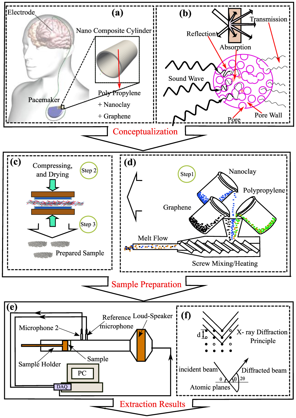
Deep brain stimulation (DBS) pacemakers are sophisticated medical devices that deliver electrical signals to targeted areas of the brain via implanted electrodes, effectively regulating abnormal brain activity and relieving symptoms of treatment-resistant neurological disorders. However, proximity to other electromagnetic equipment may introduce additional noise, which can be disruptive to individuals. To mitigate this issue, we propose a novel polymer-based nanocomposite for pacemakers for signal denoising. This research focused on the development and analysis of nanocomposites comprising polypropylene (PP) combined with montmorillonite nanoclay and graphene nanosheets (GNs). The nanocomposites were created by blending them through melting, using varying ratios of clay to GNs, with a total loading of 4 wt.%. This study focused on enhancing the signal-to-noise ratio for brain pacemakers by using nanocomposites. It investigated the noise reduction properties of PP nanocomposites, specifically in the outlet gate of the pacemaker. This research aimed to find the ideal ratio of clay to GNs in the PP matrix. X-ray diffraction (XRD) and differential scanning calorimetry (DSC) were conducted to analyze the crystalline structure and filler dispersion, as well as thermal behavior and filler–matrix interactions in the material. Scanning electron microscopy was employed to observe the dispersion of the nanofillers in the PP, and sound tube testing was conducted to evaluate the noise levels of the composites. The findings indicated that a porous structure of the nanocomposite with dispersed microspheres within the PP matrix and a long pathway facilitated increased dissipation of acoustic waves, making it suitable for denoising in brain pacemakers. Furthermore, the nanocomposite containing 2.75 wt.% of nanoclay and 1.25 wt.% of graphene components within the polypropylene matrix demonstrated a favorable signal-to-noise ratio compared to other evaluated nanocomposites.
Citation: Baraa Chasib Mezher AL Kasar, Shahab Khameneh Asl, Hamed Asgharzadeh, Seyed Jamaleddin Peighambardoust. Denoising deep brain stimulation pacemaker signals with novel polymer-based nanocomposites: Porous biomaterials for sound absorption[J]. AIMS Bioengineering, 2024, 11(2): 241-265. doi: 10.3934/bioeng.2024013
Deep brain stimulation (DBS) pacemakers are sophisticated medical devices that deliver electrical signals to targeted areas of the brain via implanted electrodes, effectively regulating abnormal brain activity and relieving symptoms of treatment-resistant neurological disorders. However, proximity to other electromagnetic equipment may introduce additional noise, which can be disruptive to individuals. To mitigate this issue, we propose a novel polymer-based nanocomposite for pacemakers for signal denoising. This research focused on the development and analysis of nanocomposites comprising polypropylene (PP) combined with montmorillonite nanoclay and graphene nanosheets (GNs). The nanocomposites were created by blending them through melting, using varying ratios of clay to GNs, with a total loading of 4 wt.%. This study focused on enhancing the signal-to-noise ratio for brain pacemakers by using nanocomposites. It investigated the noise reduction properties of PP nanocomposites, specifically in the outlet gate of the pacemaker. This research aimed to find the ideal ratio of clay to GNs in the PP matrix. X-ray diffraction (XRD) and differential scanning calorimetry (DSC) were conducted to analyze the crystalline structure and filler dispersion, as well as thermal behavior and filler–matrix interactions in the material. Scanning electron microscopy was employed to observe the dispersion of the nanofillers in the PP, and sound tube testing was conducted to evaluate the noise levels of the composites. The findings indicated that a porous structure of the nanocomposite with dispersed microspheres within the PP matrix and a long pathway facilitated increased dissipation of acoustic waves, making it suitable for denoising in brain pacemakers. Furthermore, the nanocomposite containing 2.75 wt.% of nanoclay and 1.25 wt.% of graphene components within the polypropylene matrix demonstrated a favorable signal-to-noise ratio compared to other evaluated nanocomposites.

| [1] |
Manop D, Tanghengjaroen C, Putson C, et al. (2024) The effect of polyaniline composition on the polyurethane/polyaniline composite properties: The enhancement of electrical and mechanical properties for medical tissue engineering. AIMS Mater Sci 11: 323-342. https://doi.org/10.3934/matersci.2024018 
|
| [2] |
Ananthan VB, Bernicke P, Akkermans RA, et al. (2020) Effect of porous material on trailing edge sound sources of a lifting airfoil by zonal overset-LES. J Sound Vib 480: 115386. https://doi.org/10.1016/j.jsv.2020.115386
|
| [3] |
Geyer T, Sarradj E, Fritzsche C (2010) Measurement of the noise generation at the trailing edge of porous airfoils. Exp fluids 48: 291-308. https://doi.org/10.1007/s00348-009-0739-x
|
| [4] | Shen Y, Jiang G (2016) The influence of production parameters on sound absorption of activated carbon fiber felts. J Text I 107: 1144-1149. https://doi.org/10.13475/j.fzxb.20191205805 |
| [5] |
Das P, Manna S, Behera AK, et al. (2022) Current synthesis and characterization techniques for clay-based polymer nano-composites and its biomedical applications: A review. Environ Res 212: 113534. https://doi.org/10.1016/j.envres.2022.113534
|
| [6] |
Dong Y, Bhattacharyya D (2012) Investigation on the competing effects of clay dispersion and matrix plasticisation for polypropylene/clay nanocomposites. Part II: Crystalline structure and thermo-mechanical behaviour. J Mater Sci 47: 4127-4137. http://doi.org/10.1007/s10853-012-6248-y
|
| [7] |
Mohammed L, Biglari H, Vakili-Tahami F (2023) Analyzing the buckling of FGCNT-reinforced sandwich microshells in heart pacemakers: The impact of thickness stretching on third-order shear deformation. AIP Adv 13: 075026. https://doi.org/10.1063/5.0157650
|
| [8] |
Lee PC, Kang D, Oh JT, et al. (2023) Reducing moisture absorption in polypropylene nanocomposites for automotive headlamps using hydrophobicity-modified graphene/montmorillonite. Nanomaterials-Basel 13: 1439. https://doi.org/10.3390/nano13091439
|
| [9] |
Wang J, Pei S, Yang Y, et al. (2024) Convolutional transformer-driven robust electrocardiogram signal denoising framework with adaptive parametric ReLU. Math Biosci Eng 21: 4286-4308. https://doi.org/10.3934/mbe.2024189
|
| [10] |
Zhong W, Mao L, Du W (2023) A signal quality assessment method for fetal QRS complexes detection. Math Biosci Eng 20: 7943-7956. https://doi.org/10.3934/mbe.2023344
|
| [11] |
Wen P, Zhang Y, Wen G (2023) Intelligent personalized diagnosis modeling in advanced medical system for Parkinson's disease using voice signals. Math Biosci Eng 20: 8085-8102. https://doi.org/10.3934/mbe.2023351
|
| [12] |
Justice DH, Trussell HJ, Olufsen MS (2006) Analysis of blood flow velocity and pressure signals using the multipulse method. Math Biosci Eng 3: 419-440. https://doi.org/10.3934/mbe.2006.3.419
|
| [13] |
Saurav S, Mohan A, Tabassum Z, et al. (2024) Recent trends in polymer-based nanocomposites and its application in bone tissue engineering. AIP Conference Proceedings AIP Publishing 2986: 030138. https://doi.org/10.1063/5.0197881
|
| [14] |
Sagadevan S, Schirhagl R, Rahman MZ, et al. (2023) Recent advancements in polymer matrix nanocomposites for bone tissue engineering applications. J Drug Deliv Sci Tec 82: 104313. https://doi.org/10.1016/j.jddst.2023.104313
|
| [15] |
Abbas M, Alqahtani MS, Alhifzi R (2023) Recent developments in polymer nanocomposites for bone regeneration. Int J Mol Sci 24: 3312. https://doi.org/10.3390/ijms24043312
|
| [16] |
Cingolani E, Goldhaber JI, Marbán E (2018) Next-generation pacemakers: From small devices to biological pacemakers. Nat Rev Cardiol 15: 139-150. https://doi.org/10.1038/nrcardio.2017.165
|
| [17] | Nordi TM, Gounella RH, Ginja GA, et al. (2023) Low-noise amplifier and neurostimulator in submicron CMOS for closed-loop deep-brain stimulation (CLDBS). Preprints 5: 1182. https://doi.org/10.20944/preprints202305.1182.v1 |
| [18] |
Uppu V, Mishra K, Babu LK, et al. (2019) Understanding the influence of graphene and nonclay on the microcracks developed at cryogenic temperature. AIMS Mater Sci 6: 559-566. https://doi.org/10.3934/matersci.2019.4.559
|
| [19] |
Safie NE, Azam MA (2022) Understanding the structural properties of feasible chemically reduced graphene. AIMS Mater Sci 9: 617-627. https://doi.org/10.3934/matersci.2022037
|
| [20] |
Di-Gianni A, Amerio E, Monticelli O, et al. (2008) Preparation of polymer/clay mineral nanocomposites via dispersion of silylated montmorillonite in a UV curable epoxy matrix. Appl Clay Sci 42: 116-124. https://doi.org/10.1016/j.clay.2007.12.011
|
| [21] |
Wang H, Feng Q, Liu K (2016) The dissolution behavior and mechanism of kaolinite in alkali-acid leaching process. Appl Clay Sci 132: 273-280. https://doi.org/10.1016/j.clay.2016.06.013
|
| [22] |
Zaaba NI, Foo KL, Hashim U, et al. (2017) Synthesis of graphene oxide using modified hummers method: Solvent influence. Procedia Eng 184: 469-477. https://doi.org/10.1016/j.proeng.2017.04.118
|
| [23] |
Kumar V, Singh A (2013) Polypropylene clay nanocomposites. Rev Chem Eng 29: 439-448. https://doi.org/10.1515/revce-2013-0014
|
| [24] |
Patra SC, Swain S, Senapati P, et al. (2022) Polypropylene and graphene nanocomposites: Effects of selected 2D-nanofiller's plate sizes on fundamental physicochemical properties. Inventions 8: 8. https://doi.org/10.3390/inventions8010008
|
| [25] |
Lin C, Wen G, Yin H, et al. (2022) Revealing the sound insulation capacities of TPMS sandwich panels. J Sound Vib 540: 117303. https://doi.org/10.1016/j.jsv.2022.117303
|
| [26] |
Rastegar S, Stadlbauer J, Pandhi T, et al. (2019) Measurement of signal-to-noise ratio in graphene-based passive microelectrode arrays. Electroanaly 31: 991-1001. https://doi.org/10.1002/elan.201800745
|
| [27] |
Li F, Wang R, Zheng Z, et al. (2022) A time-variant reliability analysis framework for selective laser melting fabricated lattice structures with probability and convex hybrid models. Virtual Phys Prototy 17: 841-853. https://doi.org/10.1080/17452759.2022.2074196
|
| [28] |
Naffakh M, Fernández M, Shuttleworth PS, et al. (2020) Nanocomposite materials with poly (l-lactic acid) and transition-metal dichalcogenide nanosheets 2D-TMDCs WS2. Polymers-Basel 12: 2699. https://doi.org/10.3390/polym12112699
|
| [29] |
Liu J, Chen T, Zhang Y, et al. (2019) On sound insulation of pyramidal lattice sandwich structure. Compos Struct 208: 385-394. https://doi.org/10.1016/j.compstruct.2018.10.013
|
| [30] |
Glé P, Gourdon E, Arnaud L (2011) Acoustical properties of materials made of vegetable particles with several scales of porosity. Appl Acoust 72: 249-259. http://dx.doi.org/10.1016/j.apacoust.2010.11.003
|
| [31] |
Othmani C, Taktak M, Zain A, et al. (2017) Acoustic characterization of a porous absorber based on recycled sugarcane wastes. Appl Acoust 120: 90-97. https://doi.org/10.1016/j.apacoust.2017.01.010
|
| [32] |
Pan G, Zhao Y, Xu H, et al. (2016) Acoustical and mechanical properties of thermoplastic composites from discarded carpets. Compos Part B-Eng 99: 98-105. https://doi.org/10.1016/j.compositesb.2016.06.018
|
| [33] |
Martinez L, Palessonga D, Roquefort P, et al. (2021) Development of a high temperature printable composite for microwave absorption applications. AIMS Mater Sci 8: 739-747. https://doi.org/10.3934/matersci.2021044
|
| [34] |
Rafiee M, Abidnejad R, Ranta A, et al. (2021) Exploring the possibilities of FDM filaments comprising natural fiber-reinforced biocomposites for additive manufacturing. AIMS Mater Sci 8: 524-537. https://doi.org/10.3934/matersci.2021032
|
| [35] |
Satour A, Montrésor S, Bentahar M, et al. (2014) Acoustic emission signal denoising to improve damage analysis in glass fibre-reinforced composites. Nondestruct Test Eva 29: 65-79. https://doi.org/10.1080/10589759.2013.854782
|
| [36] |
Harrouche K, Rouvaen JM, Ouaftouh M, et al. (2000) Signal-processing methods for analysing the structure of carbon-epoxy-resin composite materials. Meas Sci Technol 11: 285. https://iopscience.iop.org/article/10.1088/0957-0233/11/3/317/meta
|
| [37] |
Li Z, Xiang S, Lin Z, et al. (2021) Graphene oxide-functionalized nanocomposites promote osteogenesis of human mesenchymal stem cells via enhancement of BMP-SMAD1/5 signaling pathway. Biomaterials 277: 121082. https://doi.org/10.1016/j.biomaterials.2021.121082
|
| [38] |
Aydın G, San SE (2024) Breaking the limits of acoustic science: A review of acoustic metamaterials. Mat Sci Eng B-Adv 305: 117384. https://doi.org/10.1016/j.mseb.2024.117384
|
| [39] |
Yang X, Wen G, Jian L, et al. (2024) Archimedean spiral channel-based acoustic metasurfaces suppressing wide-band low-frequency noise at a deep subwavelength. Mater Design 238: 112703. https://doi.org/10.1016/j.matdes.2024.112703
|
| [40] |
Wen G, Zhang S, Wang H, et al. (2023) Origami-based acoustic metamaterial for tunable and broadband sound attenuation. Int J Mech Sci 239: 107872. https://doi.org/10.1016/j.ijmecsci.2022.107872
|
| [41] |
Suherman H (2019) Optimization of compression moulding parameters of multiwall carbon nanotube/synthetic graphite/epoxy nanocomposites with respect to electrical conductivity. AIMS Mater Sci 6: 621-634. https://doi.org/10.3934/matersci.2019.4.621
|
| [42] |
Kiddell S, Kazemi Y, Sorken J, et al. (2023) Influence of flash graphene on the acoustic, thermal, and mechanical performance of flexible polyurethane foam. Polym Test 119: 107919. https://doi.org/10.1016/j.polymertesting.2022.107919
|
| [43] |
Suhr J, Koratkar N, Keblinski P, et al. (2005) Viscoelasticity in carbon nanotube composites. Nat mater 4: 134-137. https://doi.org/10.1038/nmat1293
|
| [44] |
Rahbarshendi F, Baybordiani A, Asgharzadeh H, et al. (2022) The effect of graphene-based nanofillers on the structure, thermal, and mechanical properties of poly (vinyl alcohol). J Appl Polym Sci 139: e52664. https://doi.org/10.1002/app.52664
|
| [45] |
Charandabinezhad SR, Asgharzadeh H, Arsalani N (2021) Synthesis and characterization of reduced graphene oxide/magnetite/polyaniline composites as electrode materials for supercapacitors. J Mater Sci-Mater El 32: 1864-1876. https://doi.org/10.1007/s10854-020-04955-7
|
| [46] |
Asgharzadeh H, Eslami S (2019) Effect of reduced graphene oxide nanoplatelets content on the mechanical and electrical properties of copper matrix composite. J Alloy Compd 806: 553-565. https://doi.org/10.1016/j.jallcom.2019.07.183
|
| [47] |
Jafarlou H, Hassannezhad K, Asgharzadeh H, et al. (2018) Enhancement of mechanical properties of low carbon steel joints via graphene addition. Mater Sci Tech-lond 34: 455-467. https://doi.org/10.1080/02670836.2017.1407543
|
| [48] |
Abdolhosseinzadeh S, Asgharzadeh H, Seop Kim H (2015) Fast and fully-scalable synthesis of reduced graphene oxide. Sci Rep 5: 10160. https://doi.org/10.1038/srep10160
|
| [49] | Khameneh-Asl S, Namdar-Habashi M, Kianvash A, et al. (2019) Fabrication of graphene/MoS2 nanocomposite for flexible energy storage. J Nanostruct 9: 21-28. https://www.sid.ir/paper/750795/en |
| [50] | Asl SK, Namdar M (2019) Preparation of graphene/graphene oxide microsupercapacitor by using laser-scribed method. Chem Methodol 3: 183-193. https://doi.org/10.22034/chemm.2018.144016.1073 |
| [51] |
Schaldach M (1992) Materials in pacemaker technology. Electrotherapy of the Heart: Technical Aspects in Cardiac Pacing . Berlin: Springer 169-190. https://doi.org/10.1007/978-3-642-50209-5
|
| [52] |
Upadhyay S, Upadhya A, Salehi W, et al. (2021) The medical aspects of EMI effect on patients implanted with pacemakers. Mater Today Proceed 45: 5243-5248. https://doi.org/10.1016/j.matpr.2021.01.826
|
| [53] |
Cai Y, Hang Y, Zhou Y, et al. (2019) Graphene-based biosensors for detection of composite vibrational fingerprints in the Mid-infrared region. Nanomaterials-Basel 9: 1496. https://doi.org/10.3390/nano9101496
|


Figures(6) / Tables(4)

Baraa Chasib Mezher AL Kasar, Shahab Khameneh Asl, Hamed Asgharzadeh, Seyed Jamaleddin Peighambardoust. Denoising deep brain stimulation pacemaker signals with novel polymer-based nanocomposites: Porous biomaterials for sound absorption[J]. AIMS Bioengineering, 2024, 11(2): 241-265. doi: 10.3934/bioeng.2024013


 DownLoad: