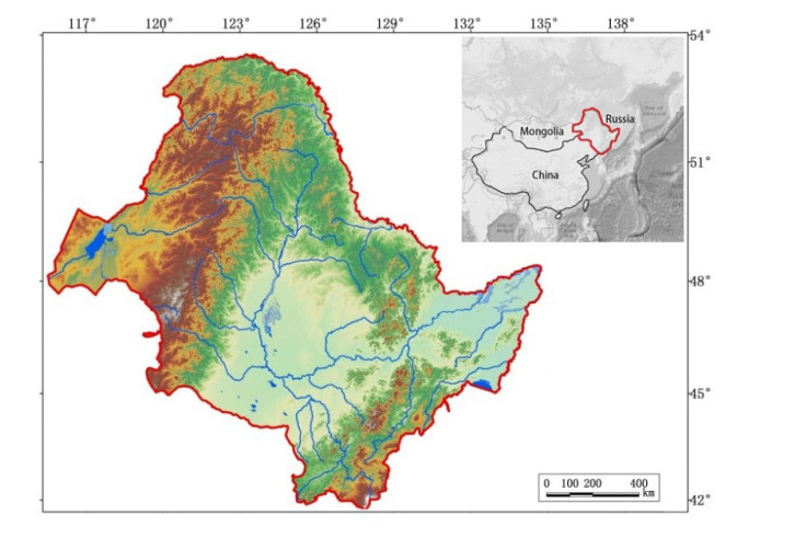
I achieved the goal of collection and storage of 1944 habitation sites in the Amur River basin by creating the ARCGIS geo-spatial database. On this basis, by visualizing the distribution of the habitation sites in six archaeological periods and four geography plates, the spatial and temporal distribution information of these sites were interpreted quantitatively. Specifically, the quantitative indicators, such as nuclear density, location of gravity center, and cultural inheritance index, revealed the spatial distribution of the habitation sites. In addition, the elevation, slope, and distance value from the river were extracted through spatial analysis of ArcGIS, revealing the characteristics of the combination of sites and geographical conditions. The analysis of vegetation and temperature-climate conditions of the Amur River basin suggests the coupling relationship between ancient settlements and the natural environment: Arable land with an average annual temperature above 4 ℃ is the area with the highest concentration of large settlements, while other woodlands, grasslands and swamps with lower average annual temperatures are the main distribution areas of small nomadic sites.
Citation: Wenqing Liu. A study on the spatial and temporal distribution of habitation sites in the Amur River Basin and its relationship with geographical environments[J]. AIMS Geosciences, 2024, 10(1): 172-195. doi: 10.3934/geosci.2024010
I achieved the goal of collection and storage of 1944 habitation sites in the Amur River basin by creating the ARCGIS geo-spatial database. On this basis, by visualizing the distribution of the habitation sites in six archaeological periods and four geography plates, the spatial and temporal distribution information of these sites were interpreted quantitatively. Specifically, the quantitative indicators, such as nuclear density, location of gravity center, and cultural inheritance index, revealed the spatial distribution of the habitation sites. In addition, the elevation, slope, and distance value from the river were extracted through spatial analysis of ArcGIS, revealing the characteristics of the combination of sites and geographical conditions. The analysis of vegetation and temperature-climate conditions of the Amur River basin suggests the coupling relationship between ancient settlements and the natural environment: Arable land with an average annual temperature above 4 ℃ is the area with the highest concentration of large settlements, while other woodlands, grasslands and swamps with lower average annual temperatures are the main distribution areas of small nomadic sites.

| [1] |
Wagner M, Tarasov P, Hosner D, et al. (2013) Mapping of the spatial and temporal distribution of archaeological sites of northern China during the Neolithic and Bronze Age. Quat Int 290: 344–357. https://doi.org/10.1016/j.quaint.2012.06.039 doi: 10.1016/j.quaint.2012.06.039

|
| [2] | Nelson SM (2001) Leadership Strategies, Economic Activity, and Interregional Interaction: Social Complexity in Northeast China. Gideon Shelach. 1999. Kluwer Academic/Plenum Publishers, New York, xv + 280 pp. $69.95 (cloth), ISBN 0-306-46090-4. Am Antiq 66: 169–170. https://doi.org/10.2307/2694330 |
| [3] |
Liu L, Chen X, Yun KL, et al. (2004) Settlement Patterns and Development of Social Complexity in the Yiluo Region, North China. J Field Archaeol 29: 75–100. https://doi.org/10.1179/jfa.2004.29.1-2.75 doi: 10.1179/jfa.2004.29.1-2.75
|
| [4] | Liu L, Chen X (2012) The Archaeology of China (From the Late Paleolithic to the Early Bronze Age). Foragers and collectors in the Pleistocene-Holocene transition (24,000–9000 cal. BP). Cambridge University Press. https://doi.org/10.1017/CBO9781139015301 |
| [5] |
Holdaway SJ, King GCP, Douglass MJ, et al. (2015) Human-environment interactions at regional scales: the complex topography hypothesis applied to surface archaeological records in Australia and North America. Archaeol Oceania 2015: 58–69. https://doi.org/10.1002/ARCO.5054 doi: 10.1002/ARCO.5054
|
| [6] |
Stewart A, Friesen TM, Keith D, et al. (2000) Archaeology and Oral History of Inuit Land Use on the Kazan River, Nunavut: A Feature-Based Approach. Arctic 53: 260–278. https://doi.org/10.14430/arctic857 doi: 10.14430/arctic857
|
| [7] |
KRISTIANSEN SM (2001) Present-day soil distribution explained by prehistoric land-use: Podzol Arenosol variation in an ancient woodland in Denmark. Geoderma 103: 273–289. https://doi.org/10.1016/S0016-7061(01)00044-1 doi: 10.1016/S0016-7061(01)00044-1
|
| [8] |
Cherry JF, Ryzewski K, Leppard TP (2012) Multi-Period Landscape Survey and Site Risk Assessment on Montserrat, West Indies. J Isl Coastal Archaeol 7: 282–302. https://doi.org/10.1080/15564894.2011.611857 doi: 10.1080/15564894.2011.611857
|
| [9] |
Hosner D, Wagner M, Tarasov PE, et al. (2016) Spatiotemporal distribution patterns of archaeological sites in China during the Neolithic and Bronze Age: An overview. Holocene 26: 1055845681. https://doi.org/10.1177/0959683616641743 doi: 10.1177/0959683616641743
|
| [10] |
Li Z, Zhu C, Wu G, et al. (2015) Spatial pattern and temporal trend of prehistoric human sites and its driving factors in Henan Province, Central China. J Geogr Sci 25: 1109–1121. https://doi.org/10.1007/s11442-015-1222-7 doi: 10.1007/s11442-015-1222-7
|
| [11] |
Yang L, Pei AP, Guo NN, et al. (2012) Spatial Modality of Prehistoric Settlement Sites in Luoyang Area. Sci Geogr Sin 32: 993–999. https://doi.org/10.13249/j.cnki.sgs.2012.08.010 doi: 10.13249/j.cnki.sgs.2012.08.010
|
| [12] |
Zhang JX, Wang XY, Yang RX, et al. (2016) Temporal-spatial distribution of archaeological sites in the Nihewan-Huliu Basin during the Paleolithic-Neolithic and Iron Age in northern China. IOP Conf Ser Earth Environ Sci 46: 012014. https://doi.org/10.1088/1755-1315/46/1/012014 doi: 10.1088/1755-1315/46/1/012014
|
| [13] |
Zheng CG, Cheng Z, Zhong YS, et al. (2008) Relationship between the temporal-spatial distribution of archaeological sites and natural environment from the Paleolithic Age to the Tang and Song Dynasties in the Three Gorges Reservoir of Chongqing area. Chin Sci Bull 53: 107–128. https://doi.org/10.1007/s11434-008-5015-6 doi: 10.1007/s11434-008-5015-6
|
| [14] |
Zheng HB, Zhou YS, Yang Q, et al. (2018) Spatial and temporal distribution of Neolithic sites in coastal China: Sea level changes, geomorphic evolution and human adaption. Sci China Earth Sci 61: 1–11. https://doi.org/10.1007/s11430-017-9121-y doi: 10.1007/s11430-017-9121-y
|
| [15] |
Feng L, Li W, Cheng Z, et al. (2013) Spatial–temporal distribution and geographic context of Neolithic cultural sites in the Hanjiang River Basin, Southern Shanxi, China. J Archaeol Sci 40: 3141–3152. https://doi.org/10.1016/j.jas.2013.04.010 doi: 10.1016/j.jas.2013.04.010
|
| [16] |
Xu J (2006) The distribution of neolithic archaeological ruins around Lianyungang area and their relation to coast lines changes. Quat Sci 26: 353–360. https://doi.org/10.3321/j.issn:1001-7410.2006.03.006 doi: 10.3321/j.issn:1001-7410.2006.03.006
|
| [17] |
Dong G, Jia X, Elston R, et al. (2013) Spatial and temporal variety of prehistoric human settlement and its influencing factors in the upper Yellow River valley, Qinghai Province, China. J Archaeol Sci 40: 2538–2546. https://doi.org/10.1016/j.jas.2012.10.002 doi: 10.1016/j.jas.2012.10.002
|
| [18] |
Lu P, Tian Y, Chen PP, et al. (2016) Spatial and temporal modes of prehistoric settlement distribution around Songshan Mountain. Acta Geogr Sin 71: 1629–1639. https://doi.org/10.11821/dlxb20160901 doi: 10.11821/dlxb20160901
|
| [19] |
Xu J, Jia Y, Ma C, et al. (2016) Geographic distribution of archaeological sites and their response to climate and environmental change between 10.0–2.8 ka BP in the Poyang Lake Basin, China. J Geogr Sci 26: 603–618. https://doi.org/10.1007/s11442-016-1288-x doi: 10.1007/s11442-016-1288-x
|
| [20] |
Li L, Wu L, Zhu C, et al. (2011) Relationship between archaeological sites distribution and environment from 1.15 Ma BP to 278 BC in Hubei Province. J Geogr Sci 21: 909–925. https://doi.org/10.1007/s11442-011-0889-7 doi: 10.1007/s11442-011-0889-7
|
| [21] |
Guo Y, Mo D, Mao L, et al. (2013) Settlement distribution and its relationship with environmental changes from the Neolithic to Shang-Zhou dynasties in northern Shandong, China. J Geogr Sci 23: 679–694. https://doi.org/10.1007/s11442-013-1037-3 doi: 10.1007/s11442-013-1037-3
|
| [22] |
Wei GU, Zhu C (2005) Distribution Feature of Neolithic Sites in North Jiangsu Province and Environmental Archaeological Research on Its Relation with Environmental Variation. Sci Geogr Sin 25: 239–243. https://doi.org/10.13249/j.cnki.sgs.2005.02.239 doi: 10.13249/j.cnki.sgs.2005.02.239
|
| [23] |
Li K, Zhu C, Jiang F, et al. (2014) Archaeological sites distribution and its physical environmental settings between ca 260–2.2 ka BP in Guizhou, Southwest China. J Geogr Sci 24: 526–538. https://doi.org/10.1007/s11442-014-1104-4 doi: 10.1007/s11442-014-1104-4
|
| [24] |
Yuan Y (2019) Cultural evolution and spatial-temporal distribution of archaeological sites from 9.5–2.3 ka BP in the Yan-Liao region, China. J Geogr Sci 29: 449–464. https://doi.org/10.1007/s11442-019-1609-y doi: 10.1007/s11442-019-1609-y
|
| [25] |
Jia X, Yi SW, Sun YF, et al.(2017) Spatial and temporal variations in prehistoric human settlement and their influencing factors on the south bank of the Xar Moron River, Northeastern China. Front Earth Sci 11: 137–147. https://doi.org/10.1007/s11707-016-0572-5 doi: 10.1007/s11707-016-0572-5
|
| [26] | Editorial committee of encyclopedia of rivers and lakes in China (2014) Encyclopedia of rivers and lakes in China. China water and power press. |
| [27] |
Bushnell GHS (1954) Prehistoric Settlement Patterns in the Viru Valley, Peru. Nature 173: 625. https://doi.org/10.1038/173625b0 doi: 10.1038/173625b0
|
| [28] | Wandsnider LA (2004) Artifact, Landscape, and Temporality in Eastern Mediterranean Archaeological Landscape Studies. In Athanassopoulos EF, Wandsnider L, eds. Mediterranean Archaeological Landscapes: Current Issues. University of Pennsylvania Press, 69–80. https://doi.org/10.9783/9781934536285.69 |
| [29] |
Costa JA, Lima Da Costa M, Kern DC (2013) Analysis of the spatial distribution of geochemical signatures for the identification of prehistoric settlement patterns in ADE and TMA sites in the lower Amazon Basin. J Archaeol Sci 40: 2771–2782. https://doi.org/10.1016/j.jas.2012.12.027 doi: 10.1016/j.jas.2012.12.027
|
| [30] |
Henry D (1989) Correlations between Reduction Strategies and Settlement Patterns. Archeol Pap Am Anthropological Assoc 1: 139–155. https://doi.org/10.1525/ap3a.1989.1.1.139 doi: 10.1525/ap3a.1989.1.1.139
|
| [31] | Danese M, Cassiodoro G, Guichon F, et al. (2016) Spatial Analysis for the Study of Environmental Settlement Patterns: The Archaeological Sites of the Santa Cruz Province. In International conference on computational science and its applications—ICCSA 2016. Lecture Notes in Computer Science, Springer, 9789. https://doi.org/10.1007/978-3-319-42089-9_14 |
| [32] |
Waters MR (2010) The Impact of Fluvial Processes and Landscape Evolution on Archaeological Sites and Settlement Patterns Along the San Xavier Reach of the Santa Cruz River, Arizona. Geoarchaeology 3: 205–219. https://doi.org/10.1002/gea.3340030304 doi: 10.1002/gea.3340030304
|
| [33] | Davies MH (2006) An archaeological analysis of later prehistoric settlement and society in Perthshire and Stirlingshire. Durham University. |
| [34] | Heilongjiang Provincial Institute of Archaeology (2004) Qixing river: Investigation and Survey Report on Ancient Sites in the Sanjiang Plain. Beijing, Science Press. |
| [35] | Heilongjiang Provincial Institute of Archaeology (2009) Shangjing City of Balhae state: Archaeological Excavation Survey Report from 1998 to 2007. Beijing: Cultural Relics Publishing House. |
| [36] | Feng EX, Wu S (2017) Investigation and excavation of the Liaojin nomadic camp Site Groups in Qian'an County Houming area, Jilin Province. Archaeology 2017: 28–43. |
| [37] | Wang MF (1996) A study on the settlement geography of Bronze period in Jilin province. J Chin Hist Geogr 1996: 27–41. https://doi.org/CNKI: SUN: ZGLD.0.1996-04-001 |
| [38] | Qiu SW, Wang XK, Zhang SQ, et al. (2012) The evolution of ancient great lakes in Song liao plain and the formation of the plain. Quat Sci 32: 1011–1021. https://doi.org/ https://doi.org/10.3969/j.issn.1001-7410.2012.05.17 |
| [39] |
Liu WQ, Liu DP (2019) Interpretation of Settlement Space Organization Information from the Perspective of Landscape Archaeology: Taking the Han Wei Settlement Site in the Sanjiang Plain as an Example. J Archit 2019: 83–90. https://doi.org/10.3969/j.issn.0529-1399.2019.11.012 doi: 10.3969/j.issn.0529-1399.2019.11.012
|
| [40] |
Zhang XY, Xie YW, Zhu LQ, et al. (2023) Spatial and temporal characteristics of cultural sites and its natural environment in Xinjiang in historical periods. J Arid Land Resour Environ 37: 109–116. https://doi.org/10.13448/j.cnki.jalre.2023.093 doi: 10.13448/j.cnki.jalre.2023.093
|
| [41] |
Luan FM, Wang F, Xiong HG (2017) Spatio-temporal distribution of cultural sites and geographic backgrounds in the Ili River Valley. Arid Land Geogr 40: 212–221. https://doi.org/10.13826/j.cnki.cn65-1103/x.2017.01.027 doi: 10.13826/j.cnki.cn65-1103/x.2017.01.027
|
| [42] |
Zou JJ, Zhang YS, Liu T, et al. (2022) Spatio-temporal Evolution of Cultural Sites and Influences Analysis of Geomorphology in Historical Period of Zhejiang Province. J Hangzhou Norm Univ 21: 190–203. https://doi.org/10.19926/j.cnki.issn.1674-232X.2022.02.013 doi: 10.19926/j.cnki.issn.1674-232X.2022.02.013
|
| [43] |
Vita-Finzi C, Higgs ES, Sturdy D, et al. (1970) Prehistoric Economy in the Mount Carmel Area of Palestine: Site Catchment Analysis. Proc Prehistoric Soc 36: 1–37. https://doi.org/10.1017/S0079497X00013074 doi: 10.1017/S0079497X00013074
|


Figures(16) / Tables(3)

Wenqing Liu. A study on the spatial and temporal distribution of habitation sites in the Amur River Basin and its relationship with geographical environments[J]. AIMS Geosciences, 2024, 10(1): 172-195. doi: 10.3934/geosci.2024010


 DownLoad: