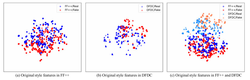
Most existing deepfake detection methods often fail to maintain their performance when confronting new test domains. To address this issue, we propose a generalizable deepfake detection system to implement style diversification by alternately learning the domain generalization (DG)-based detector and the stylized fake face synthesizer (SFFS). For the DG-based detector, we first adopt instance normalization- and batch normalization-based structures to extract the local and global image statistics as the style and content features, which are then leveraged to obtain the more diverse feature space. Subsequently, contrastive learning is used to emphasize common style features while suppressing domain-specific ones, and adversarial learning is performed to obtain the domain-invariant features. These optimized features help the DG-based detector to learn generalized classification features and also encourage the SFFS to simulate possibly unseen domain data. In return, the samples generated by the SFFS would contribute to the detector's learning of more generalized features from augmented training data. Such a joint learning and training process enhances both the detector's and the synthesizer's feature representation capability for generalizable deepfake detection. Experimental results demonstrate that our method outperforms the state-of-the-art competitors not only in intra-domain tests but particularly in cross-domain tests.
Citation: Jicheng Li, Beibei Liu, Hao-Tian Wu, Yongjian Hu, Chang-Tsun Li. Jointly learning and training: using style diversification to improve domain generalization for deepfake detection[J]. Electronic Research Archive, 2024, 32(3): 1973-1997. doi: 10.3934/era.2024090
Most existing deepfake detection methods often fail to maintain their performance when confronting new test domains. To address this issue, we propose a generalizable deepfake detection system to implement style diversification by alternately learning the domain generalization (DG)-based detector and the stylized fake face synthesizer (SFFS). For the DG-based detector, we first adopt instance normalization- and batch normalization-based structures to extract the local and global image statistics as the style and content features, which are then leveraged to obtain the more diverse feature space. Subsequently, contrastive learning is used to emphasize common style features while suppressing domain-specific ones, and adversarial learning is performed to obtain the domain-invariant features. These optimized features help the DG-based detector to learn generalized classification features and also encourage the SFFS to simulate possibly unseen domain data. In return, the samples generated by the SFFS would contribute to the detector's learning of more generalized features from augmented training data. Such a joint learning and training process enhances both the detector's and the synthesizer's feature representation capability for generalizable deepfake detection. Experimental results demonstrate that our method outperforms the state-of-the-art competitors not only in intra-domain tests but particularly in cross-domain tests.

| [1] | F. Chollet, Xception: Deep learning with depthwise separable convolutions, in 2017 IEEE Conference on Computer Vision and Pattern Recognition (CVPR), (2017), 1800–1807. https://doi.org/10.1109/CVPR.2017.195 |
| [2] |
B. Bayar, M. C. Stamm, Constrained convolutional neural networks: a new approach towards general purpose image manipulation detection, IEEE Trans. Inf. Forensics Secur., 13 (2018), 2691–2706. https://doi.org/10.1109/TIFS.2018.2825953 doi: 10.1109/TIFS.2018.2825953

|
| [3] | R. Durall, M. Keuper, J. Keuper, Watch your up-convolution: CNN based generative deep neural networks are failing to reproduce spectral distributions, in 2020 IEEE/CVF Conference on Computer Vision and Pattern Recognition (CVPR), (2020), 7887–7896. https://doi.org/10.1109/CVPR42600.2020.00791 |
| [4] | Y. Qian, G. Yin, L. Sheng, Z. Chen, J. Shao, Thinking in frequency: face forgery detection by mining frequency-aware clues, in Computer Vision – ECCV 2020, Springer, (2020), 86–103. https://doi.org/10.1007/978-3-030-58610-2_6 |
| [5] | H. Zhao, W. Zhou, D. Chen, T. Wei, W. Zhang, N. Yu, Multi-attentional deepfake detection, in 2021 IEEE/CVF Conference on Computer Vision and Pattern Recognition (CVPR), (2021), 2185–2194. https://doi.org/10.1109/CVPR46437.2021.00222 |
| [6] | Y. Luo, Y. Zhang, J. Yan, W. Liu, Generalizing face forgery detection with high-frequency features, in Proceedings of the IEEE/CVF Conference on Computer Vision and Pattern Recognition (CVPR), (2021), 16317–16326. |
| [7] |
J. Yang, A. Li, S. Xiao, W. Lu, X. Gao, Mtd-net: learning to detect deepfakes images by multi-scale texture difference, IEEE Trans. Inf. Forensics Secur., 16 (2021), 4234–4245. https://doi.org/10.1109/TIFS.2021.3102487 doi: 10.1109/TIFS.2021.3102487
|
| [8] |
B. Chen, W. Tan, Y. Wang, G. Zhao, Distinguishing between natural and GAN-generated face images by combining global and local features, Chin. J. Electron., 31 (2022), 59–67. https://doi.org/10.1049/cje.2020.00.372 doi: 10.1049/cje.2020.00.372
|
| [9] |
G. Li, X. Zhao, Y. Cao, Forensic symmetry for deepfakes, IEEE Trans. Inf. Forensics Secur., 18 (2023), 1095–1110. https://doi.org/10.1109/TIFS.2023.3235579 doi: 10.1109/TIFS.2023.3235579
|
| [10] | P. Zhou, X. Han, V. I. Morariu, L. S. Davis, Two-stream neural networks for tampered face detection, in 2017 IEEE Conference on Computer Vision and Pattern Recognition Workshops (CVPRW), IEEE, (2017), 1831–1839. https://doi.org/10.1109/CVPRW.2017.229 |
| [11] | L. Li, J. Bao, T. Zhang, H. Yang, D. Chen, F. Wen, et al., Face x-ray for more general face forgery detection, in Proceedings of the IEEE/CVF Conference on Computer Vision and Pattern Recognition (CVPR), (2020), 5001–5010. |
| [12] |
B. Chen, X. Liu, Y. Zheng, G. Zhao, Y. Q. Shi, A robust GAN-generated face detection method based on dual-color spaces and an improved xception, IEEE Trans. Circuits Syst. Video Technol., 32 (2022), 3527–3538. https://doi.org/10.1109/TCSVT.2021.3116679 doi: 10.1109/TCSVT.2021.3116679
|
| [13] | S. Chen, T. Yao, Y. Chen, S. Ding, J. Li, R. Ji, Local relation learning for face forgery detection, in AAAI Technical Track on Computer Vision I, 35 (2021), 1081–1088. https://doi.org/10.1609/aaai.v35i2.16193 |
| [14] | Y. Zheng, J. Bao, D. Chen, M. Zeng, F. Wen, Exploring temporal coherence for more general video face forgery detection, in 2021 IEEE/CVF International Conference on Computer Vision (ICCV), (2021), 15024–15034. https://doi.org/10.1109/ICCV48922.2021.01477 |
| [15] |
G. Pang, B. Zhang, Z. Teng, Z. Qi, J. Fan, Mre-net: Multi-rate excitation network for deepfake video detection, IEEE Trans. Circuits Syst. Video Technol., 33 (2023), 3663–3676. https://doi.org/10.1109/TCSVT.2023.3239607 doi: 10.1109/TCSVT.2023.3239607
|
| [16] |
B. Chen, T. Li, W. Ding, Detecting deepfake videos based on spatiotemporal attention and convolutional LSTM, Inf. Sci., 601 (2022), 58–70. https://doi.org/10.1016/j.ins.2022.04.014 doi: 10.1016/j.ins.2022.04.014
|
| [17] | H. Liu, X. Li, W. Zhou, Y. Chen, Y. He, H. Xue, et al., Spatial-phase shallow learning: rethinking face forgery detection in frequency domain, in Proceedings of the IEEE/CVF Conference on Computer Vision and Pattern Recognition (CVPR), (2021), 772–781. |
| [18] | J. Cao, C. Ma, T. Yao, S. Chen, S. Ding, X. Yang, End-to-end reconstruction-classification learning for face forgery detection, in Proceedings of the IEEE/CVF Conference on Computer Vision and Pattern Recognition (CVPR), (2022), 4113–4122. |
| [19] |
P. Yu, J. Fei, Z. Xia, Z. Zhou, J. Weng, Improving generalization by commonality learning in face forgery detection, IEEE Trans. Inf. Forensics Secur., 17 (2022), 547–558. https://doi.org/10.1109/TIFS.2022.3146781 doi: 10.1109/TIFS.2022.3146781
|
| [20] |
A. Luo, C. Kong, J. Huang, Y. Hu, X. Kang, A. C. Kot, Beyond the prior forgery knowledge: mining critical clues for general face forgery detection, IEEE Trans. Inf. Forensics Secur., 19 (2024), 1168–1182. https://doi.org/10.1109/TIFS.2023.3332218 doi: 10.1109/TIFS.2023.3332218
|
| [21] |
J. Hu, X. Liao, W. Wang, Z. Qin, Detecting compressed deepfake videos in social networks using frame-temporality two-stream convolutional network, IEEE Trans. Circuits Syst. Video Technol., 32 (2022), 1089–1102. https://doi.org/10.1109/TCSVT.2021.3074259 doi: 10.1109/TCSVT.2021.3074259
|
| [22] | T. Wang, K. P. Chow, Noise based deepfake detection via multi-head relative-interaction, in Proceedings of the AAAI Conference on Artificial Intelligence, 37 (2023), 14548–14556. https://doi.org/10.1609/aaai.v37i12.26701 |
| [23] | Y. Li, S. Lyu, Exposing deepfake videos by detecting face warping artifacts, in 2019 IEEE Conference on Computer Vision and Pattern Recognition Workshops, IEEE, (2019), 46–52. |
| [24] | T. Zhao, X. Xu, M. Xu, H. Ding, Y. Xiong, W. Xia, Learning self-consistency for deepfake detection, in 2021 IEEE/CVF International Conference on Computer Vision (ICCV), (2021), 15003–15013. https://doi.org/10.1109/ICCV48922.2021.01475 |
| [25] | K. Shiohara, T. Yamasaki, Detecting deepfakes with self-blended images, in 2022 IEEE/CVF Conference on Computer Vision and Pattern Recognition (CVPR), (2022), 18699–18708. https://doi.org/10.1109/CVPR52688.2022.01816 |
| [26] |
H. Chen, Y. Lin, B. Li, S. Tan, Learning features of intra-consistency and inter-diversity: keys toward generalizable deepfake detection, IEEE Trans. Circuits Syst. Video Technol., 33 (2023), 1468–1480. https://doi.org/10.1109/TCSVT.2022.3209336 doi: 10.1109/TCSVT.2022.3209336
|
| [27] | A. Rossler, D. Cozzolino, L. Verdoliva, C. Riess, J. Thies, M. Niessner Faceforensics++: Learning to detect manipulated facial images, in 2019 IEEE/CVF International Conference on Computer Vision (ICCV), (2019), 1–11. https://doi.org/10.1109/ICCV.2019.00009 |
| [28] | B. Dolhansky, J. Bitton, B. Pflaum, J. Lu, R. Howes, M. Wang, et al., The deepfake detection challenge (DFDC) dataset, preprint, arXiv: 2006.07397. |
| [29] | L. V. der Maaten, G. Hinton, Visualizing data using t-SNE, J. Mach. Learn. Res., 9 (2008), 2579–2605. Available from: https://www.jmlr.org/papers/volume9/vandermaaten08a/vandermaaten08a.pdf?fbcl. |
| [30] | Z. Wang, Z. Wang, Z. Yu, W. Deng, J. Li, T. Gao, Domain generalization via shuffled style assembly for face anti-spoofing, in 2022 IEEE/CVF Conference on Computer Vision and Pattern Recognition (CVPR), (2022), 4113–4123. https://doi.org/10.1109/CVPR52688.2022.00409 |
| [31] | Y. Ganin, V. Lempitsky, Unsupervised domain adaptation by backpropagation, in Proceedings of the 32nd International Conference on Machine Learning, 37 (2015), 1180–1189. Available from: http://proceedings.mlr.press/v37/ganin15.html. |
| [32] |
Y. Wang, L. Qi, Y. Shi, Y. Gao, Feature-based style randomization for domain generalization, IEEE Trans. Circuits Syst. Video Technol., 32 (2022), 5495–5509. https://doi.org/10.1109/TCSVT.2022.3152615 doi: 10.1109/TCSVT.2022.3152615
|
| [33] |
S. Lin, C. T. Li, A. C. Kot, Multi-domain adversarial feature generalization for person re-identification, IEEE Trans. Image Process., 30 (2021), 1596–1607. https://doi.org/10.1109/TIP.2020.3046864 doi: 10.1109/TIP.2020.3046864
|
| [34] | H. Nam, H. Lee, J. Park, W. Yoon, D. Yoo, Reducing domain gap by reducing style bias, in Proceedings of the IEEE/CVF Conference on Computer Vision and Pattern Recognition (CVPR), (2021), 8690–8699. |
| [35] | Q. Zhou, K. Y. Zhang, T. Yao, X. Lu, R. Yi, S. Ding, et al., Instance-aware domain generalization for face anti-spoofing, in 2023 IEEE/CVF Conference on Computer Vision and Pattern Recognition (CVPR), (2023), 20453–20463. https://doi.org/10.1109/CVPR52729.2023.01959 |
| [36] | X. Huang, S. Belongie, Arbitrary style transfer in real-time with adaptive instance normalization, in 2017 IEEE International Conference on Computer Vision (ICCV), (2017), 1510–1519. https://doi.org/10.1109/ICCV.2017.167 |
| [37] | T. Karras, S. Laine, T. Aila, A style-based generator architecture for generative adversarial networks, in 2019 IEEE/CVF Conference on Computer Vision and Pattern Recognition (CVPR), (2019), 4396–4405. https://doi.org/10.1109/CVPR.2019.00453 |
| [38] | Z. Liu, Y. Lin, Y. Cao, H. Hu, Y. Wei, Z. Zhang, et al., Swin transformer: hierarchical vision transformer using shifted windows, in Proceedings of the IEEE/CVF International Conference on Computer Vision (ICCV), (2021), 10012–10022. |
| [39] | Z. Xie, Z. Zhang, Y. Cao, Y. Lin, J. Bao, Z. Yao, et al., Simmim: a simple framework for masked image modeling, in Proceedings of the IEEE/CVF Conference on Computer Vision and Pattern Recognition (CVPR), (2022), 9653–9663. |
| [40] | D. E. King, Dlib-ml: a machine learning toolkit, J. Mach. Learn. Res., 10 (2009), 1755–1758. Available from: https://www.jmlr.org/papers/volume10/king09a/king09a.pdf. |
| [41] |
Z. Guo, G. Yang, J. Chen, X. Sun, Exposing deepfake face forgeries with guided residuals, IEEE Trans. Multimedia, 25 (2023), 8458–8470. https://doi.org/10.1109/TMM.2023.3237169 doi: 10.1109/TMM.2023.3237169
|
| [42] | M. Schroepfer, Creating a data set and a challenge for deepfakes, in Facebook Artificial Intelligence, 5 (2019). Available from: https://ai.facebook.com/blog/deepfake-detection-challenge. |
| [43] | Y. Li, X. Yang, P. Sun, H. Qi, S. Lyu, Celeb-df: a large-scale challenging dataset for deepfake forensics, in Proceedings of the IEEE/CVF Conference on Computer Vision and Pattern Recognition (CVPR), (2020), 3207–3216. |
| [44] | L. Jiang, R. Li, W. Wu, C. Qian, C. C. Loy, Deeperforensics-1.0: a large-scale dataset for real-world face forgery detection, in 2020 IEEE/CVF Conference on Computer Vision and Pattern Recognition (CVPR), (2020), 2886–2895. https://doi.org/10.1109/CVPR42600.2020.00296 |
| [45] | G. Bradski, The opencv library, in Dr. Dobb's Journal: Software Tools for the Professional Programmer, 25 (2000), 120–123. |
| [46] | R. R. Selvaraju, M. Cogswell, A. Das, R. Vedantam, D. Parikh, D. Batra, Grad-cam: visual explanations from deep networks via gradient-based localization, in 2017 IEEE International Conference on Computer Vision (ICCV), (2017), 618–626. https://doi.org/10.1109/ICCV.2017.74 |
| [47] | K. He, X. Zhang, S. Ren, J. Sun, Deep residual learning for image recognition, in Proceedings of the IEEE Conference on Computer Vision and Pattern Recognition (CVPR), (2016), 770–778. |
| [48] | M. Tan, Q. Le, Efficientnet: rethinking model scaling for convolutional neural networks, in Proceedings of the 36th International Conference on Machine Learning, (2019), 6105–6114. |


Figures(6) / Tables(9)
Jicheng Li, Beibei Liu, Hao-Tian Wu, Yongjian Hu, Chang-Tsun Li. Jointly learning and training: using style diversification to improve domain generalization for deepfake detection[J]. Electronic Research Archive, 2024, 32(3): 1973-1997. doi: 10.3934/era.2024090


 DownLoad: