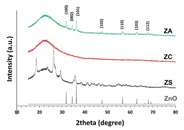
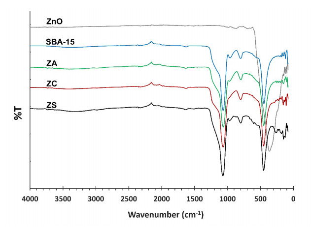
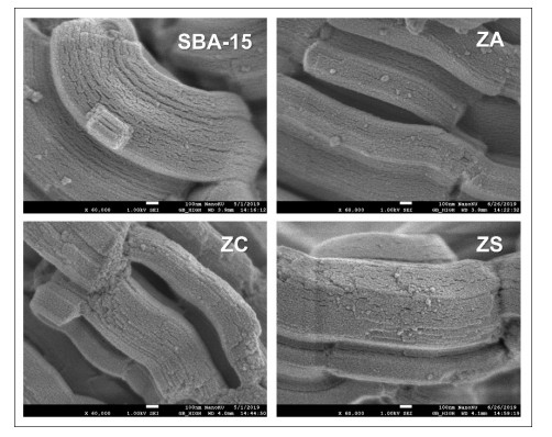
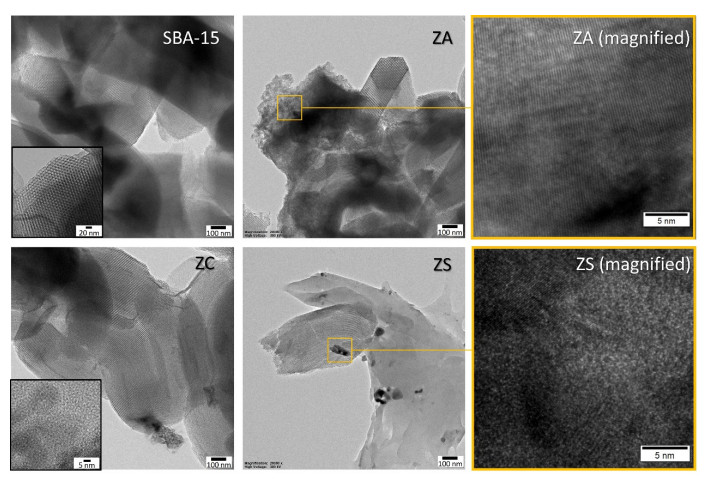
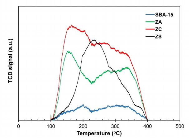
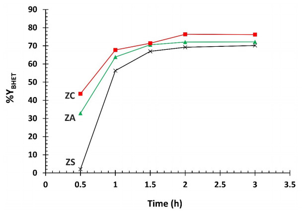
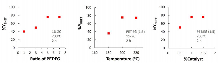
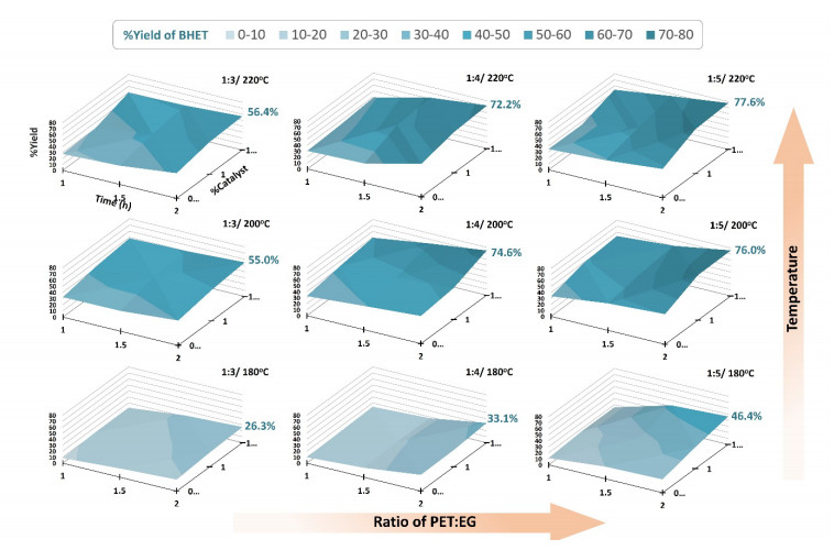
Novel catalysts for recycling PET bottles into monomers have been developed by depositing zinc onto the surface of SBA-15, mitigating ZnO catalyst agglomeration in glycolysis separation processes to enhance reaction yields. Various zinc compounds (Zn(OAc)2, ZnCl2, and ZnSO4) were employed as substrates for catalyst design on the porous, high-surface-area material SBA-15 via impregnation. The presence of distinct Zn species on SBA-15 was confirmed through XRD and EDS analyses. The acidity of the catalyst, a crucial factor in the PET glycolysis process, was assessed using different Zn-containing precursors. NH3-TPD measurement has revealed the highest acidity in ZnCl2, followed by Zn(OAc)2 and ZnSO4, respectively. Glycolysis reactions with a PET:EG ratio of 1:5 and a 1% catalyst at 200℃ for 2 hours revealed the catalytic efficacy of zinc-deposited compounds in the sequence ZnCl2 > Zn(OAc)2 > ZnSO4. Surprisingly, the ZnCl2 catalyst produced the highest yield of bis-2-hydroxyethyl terephthalate (BHET) at 75% and displayed exceptional recycling capability over three cycles, contributing significantly to resource recovery objectives aligned with the Sustainable Development Goals (SDGs).
Citation: Pailin Srisuratsiri, Ketsarin Chantarasunthon, Wanutsanun Sudsai, Pichet Sukprasert, Laksamee Chaicharoenwimolkul Chuaitammakit, Wissawat Sakulsaknimitr. Sustainable plastic bottle recycling: employing zinc-deposited SBA-15 as a catalyst for glycolysis of polyethylene terephthalate[J]. AIMS Environmental Science, 2024, 11(1): 90-106. doi: 10.3934/environsci.2024006
Novel catalysts for recycling PET bottles into monomers have been developed by depositing zinc onto the surface of SBA-15, mitigating ZnO catalyst agglomeration in glycolysis separation processes to enhance reaction yields. Various zinc compounds (Zn(OAc)2, ZnCl2, and ZnSO4) were employed as substrates for catalyst design on the porous, high-surface-area material SBA-15 via impregnation. The presence of distinct Zn species on SBA-15 was confirmed through XRD and EDS analyses. The acidity of the catalyst, a crucial factor in the PET glycolysis process, was assessed using different Zn-containing precursors. NH3-TPD measurement has revealed the highest acidity in ZnCl2, followed by Zn(OAc)2 and ZnSO4, respectively. Glycolysis reactions with a PET:EG ratio of 1:5 and a 1% catalyst at 200℃ for 2 hours revealed the catalytic efficacy of zinc-deposited compounds in the sequence ZnCl2 > Zn(OAc)2 > ZnSO4. Surprisingly, the ZnCl2 catalyst produced the highest yield of bis-2-hydroxyethyl terephthalate (BHET) at 75% and displayed exceptional recycling capability over three cycles, contributing significantly to resource recovery objectives aligned with the Sustainable Development Goals (SDGs).

| [1] |
Leslie HA, van Velzen MJM, Brandsma SH, et al. (2021) Discovery and quantification of plastic particle pollution in human blood. Environ Int 163: 107199. https://doi.org/10.1016/j.envint.2022.107199 doi: 10.1016/j.envint.2022.107199

|
| [2] | Raheem AB, Noor ZZ, Hassan A, et al. (2019) Current developments in chemical recycling of post-consumer polyethylene terephthalate wastes for new materials production: A review. J Clean Prod. 225: 1052–1064. https://doi.org/10.1016/j.jclepro.2019.04.019 |
| [3] |
Benyathiar P, Kumar P, Carpenter G, et at. (2022) Polyethylene Terephthalate (PET) Bottle-to-Bottle Recycling for the Beverage Industry: A Review. Polymers 14: 2366. https://doi.org/10.3390/polym14122366 doi: 10.3390/polym14122366
|
| [4] |
Zhang Q, Huang R, Yao H, et al. (2021) Removal of Zn2+from polyethylene terephthalate (PET) glycolytic monomers by sulfonic acid cation exchange resin. J Environ Chem Eng 9:105326. https://doi.org/10.1016/j.jece.2021.105326 doi: 10.1016/j.jece.2021.105326
|
| [5] |
Vieira CO, Grice JE, Roberts MS, et al. (2018) ZnO:SBA-15 nanocomposites for potential use in sunscreen: Preparation, properties, human skin penetration and toxicity. Skin Pharmacol Physiol 32: 32–42. https://doi.org/10.1159/000491758 doi: 10.1159/000491758
|
| [6] | Imran M, Kim DH, Al-Masry WA, et al. (2013) Manganese-, cobalt-, and zinc-based mixed-oxide spinels as novel catalysts for the chemical recycling of poly(ethylene terephthalate) via glycolysis. Polym Degrad Stab. 98: 904–915. https://doi.org/10.1016/j.polymdegradstab.2013.01.007 |
| [7] | Kawkumpa S, Saisema T, Seoob O, et al. (2019) Synthesis of polyurethane from glycolysis product of PET using ZnO as catalyst. RMUTSB Acad J 7: 29–39 https://li01.tci-thaijo.org/index.php/rmutsb-sci/article/view/150479 |
| [8] |
Shen Z, Zhou H, Chen H, et al. (2018) Synthesis of Nano-Zinc Oxide Loaded on Mesoporous Silica by Coordination Effect and Its Photocatalytic Degradation Property of Methyl Orange. Nanomater 8: 317. https://doi.org/10.3390/nano8050317 doi: 10.3390/nano8050317
|
| [9] | Nguyen QNK, Yen NT, Hau ND, et al. (2020) Synthesis and Characterization of Mesoporous Silica SBA-15 and ZnO/SBA-15 Photocatalytic Materials from the Ash of Brickyards. J Chem Article ID 8456194, 8 pages: https://doi.org/10.1155/2020/8456194 |
| [10] | Wen H, Zhou X, Shen Z, et al. (2019) Synthesis of ZnO nanoparticles supported on mesoporous SBA-15 with coordination effect -assist for anti-bacterial assessment. Colloids Surf. B 181: 285–294. https://doi.org/10.1016/j.colsurfb.2019.05.055 |
| [11] | Bhuyan D, Saikia M, Saikia L. (2018) ZnO nanoparticles embedded in SBA-15 as an efficient heterogeneous catalyst for the synthesis of dihydropyrimidinones via Biginelli condensation reaction. Microporous Mesoporous Mater 256: 39–48. https://doi.org/10.1016/j.micromeso.2017.06.052 |
| [12] |
Pal N, Paul M, Bhaumik A. (2011) Highly ordered Zn-doped mesoporous silica: An efficient catalyst for transesterification reaction. J Solid State Chem 184: 1805–1812. https://doi.org/10.1016/j.jssc.2011.05.033 doi: 10.1016/j.jssc.2011.05.033
|
| [13] |
Nagvenkar A, Naik S, Fernandes J. (2015) Zinc oxide as a solid acid catalyst for esterification reaction. Catal Commun 65: 20–23. https://doi.org/10.1016/j.catcom.2015.02.009 doi: 10.1016/j.catcom.2015.02.009
|
| [14] |
Yao H, Liu L, Yan D, et al. (2022) Colorless BHET obtained from PET by modified mesoporous catalyst ZnO/SBA-15. Chem Eng Sci 248: 117109. https://doi.org/10.1016/j.ces.2021.117109 doi: 10.1016/j.ces.2021.117109
|
| [15] |
Datta B, Pasha MA. (2013) Silica-ZnCl2: An Efficient Catalyst for the Synthesis of 4-Methylcoumarins. ISRN Org Chem 13: 1–5. https://doi.org/10.1155/2013/132794 doi: 10.1155/2013/132794
|
| [16] |
Lin CC, Li YY. (2009) Synthesis of ZnO nanowires by thermal decomposition of zinc acetate dihydrate. Mater Chem Phys 113: 334–337. https://doi.org/10.1016/j.matchemphys.2008.07.070 doi: 10.1016/j.matchemphys.2008.07.070
|
| [17] |
Jones F, Tran H, Lindberg D, et al. (2013) Thermal Stability of Zinc Compounds. Energy and Fuels 27: 5663–5669. https://doi.org/10.1021/ef400505u doi: 10.1021/ef400505u
|
| [18] |
Moosavi A, Sarrafi M, Aghaei A, et al. (2012) Synthesis of mesoporous ZnO/SBA-15 composite via sonochemical route. Micro Nano Lett 7: 130–133. DOI: 10.1049/mnl.2011.0461 doi: 10.1049/mnl.2011.0461
|
| [19] |
Saha J, Podder J. (2011) Crystallization Of Zinc Sulphate Single Crystals And Its Structural, Thermal And Optical Characterization. J Bangladesh Acad Sci 35: 203–210. https://doi.org/10.3329/jbas.v35i2.9426 doi: 10.3329/jbas.v35i2.9426
|
| [20] |
Foad Raji MP. (2013) Study of Hg(Ⅱ) species removal from aqueous solution using hybrid ZnCl2-MCM-41 adsorbent. Appl Surf Sci 282: 415–424. https://doi.org/10.1016/j.apsusc.2013.05.145 doi: 10.1016/j.apsusc.2013.05.145
|
| [21] |
Jiang Q, Wu ZY, Wang YM, et al. (2006) Fabrication of photoluminescent ZnO/SBA-15 through directly dispersing zinc nitrate into the as-prepared mesoporous silica occluded with template. J Mater Chem 16: 1536–1542. https://doi.org/10.1039/B516061H doi: 10.1039/B516061H
|
| [22] |
Tay YY, Li S, Sun CQ, et al. (2006) Size dependence of Zn 2p 32 binding energy in nanocrystalline ZnO. Appl Phys Lett 88: 173118. https://doi.org/10.1063/1.2198821 doi: 10.1063/1.2198821
|
| [23] | Winiarski J, Tylus W, Winiarska K, et al. (2018) XPS and FT-IR Characterization of Selected Synthetic Corrosion Products of Zinc Expected in Neutral Environment Containing Chloride Ions. J Spectrosc Article ID 2079278. https://doi.org/10.1155/2018/2079278 |
| [24] |
Miyao T, Kitai M, Ogita T, et al. (2002) Generation of new acidic sites by dispersing zinc oxide fine particles on silica. Zeitschrift fur Phys Chemie 216: 931–939. https://doi.org/10.1524/zpch.2002.216.7.931 doi: 10.1524/zpch.2002.216.7.931
|
| [25] |
Gabrienko AA, Arzumanov SS, Toktarev AV, et al. (2017) Different Efficiency of Zn2+ and ZnO Species for Methane Activation on Zn-Modified Zeolite. ACS Catal 7: 1818–1830. https://doi.org/10.1021/acscatal.6b03036 doi: 10.1021/acscatal.6b03036
|
| [26] |
Zhiyong Y, Bensimon M, Sarria V, et al. (2007) ZnSO4-TiO2 doped catalyst with higher activity in photocatalytic processes. Appl Catal B Environ 76: 185–195. https://doi.org/10.1016/j.apcatb.2007.05.025 doi: 10.1016/j.apcatb.2007.05.025
|
| [27] | Cychosz KA, Thommes M. (2018) Progress in the Physisorption Characterization of Nanoporous Gas Storage Materials. Engineering. 4: 559–566. https://doi.org/10.1016/j.eng.2018.06.001 |
| [28] |
Lao-Ubol S, Khunlad R, Larpkiattaworn S, et al. (2016) Preparation, Characterization and Catalytic Performance of ZnO-SBA-15 Catalysts. Key Eng Mater 690: 212–217. https://doi.org/10.4028/www.scientific.net/KEM.690.212 doi: 10.4028/www.scientific.net/KEM.690.212
|
| [29] |
Liu J, Liu Y, Liu H, et al. (2021) Silicalite-1 Supported ZnO as an Efficient Catalyst for Direct Propane Dehydrogenation. ChemCatChem 13: 4780–4786. https://doi.org/10.1002/cctc.202101069 doi: 10.1002/cctc.202101069
|
| [30] |
Liu G, Liu J, He N, Miao C, et al. (2018) Silicalite-1 zeolite acidification by zinc modification and its catalytic properties for isobutane conversion. RSC Adv 8: 18663–18671. https://doi.org/10.1039/C8RA02467G doi: 10.1039/C8RA02467G
|
| [31] | Xin J, Zhang Q, Huang J, et al. (2021) Progress in the catalytic glycolysis of polyethylene terephthalate. J Environ Manage. 296: 113267. https://doi.org/10.1016/j.jenvman.2021.113267 |
| [32] |
Al-Sabagh AM, Yehia FZ, Eshaq G, et al. (2016) Greener routes for recycling of polyethylene terephthalate. Egypt J Pet 25: 53–64. https://doi.org/10.1016/j.ejpe.2015.03.001 doi: 10.1016/j.ejpe.2015.03.001
|
| [33] |
Imran M, Kim BK, Han M, et al. (2010) Sub- and supercritical glycolysis of polyethylene terephthalate (PET) into the monomer bis(2-hydroxyethyl) terephthalate (BHET). Polym Degrad Stab 95:1686–1693. https://doi.org/10.1016/j.polymdegradstab.2010.05.026 doi: 10.1016/j.polymdegradstab.2010.05.026
|
Figures(8) / Tables(3)

Pailin Srisuratsiri, Ketsarin Chantarasunthon, Wanutsanun Sudsai, Pichet Sukprasert, Laksamee Chaicharoenwimolkul Chuaitammakit, Wissawat Sakulsaknimitr. Sustainable plastic bottle recycling: employing zinc-deposited SBA-15 as a catalyst for glycolysis of polyethylene terephthalate[J]. AIMS Environmental Science, 2024, 11(1): 90-106. doi: 10.3934/environsci.2024006


 DownLoad: