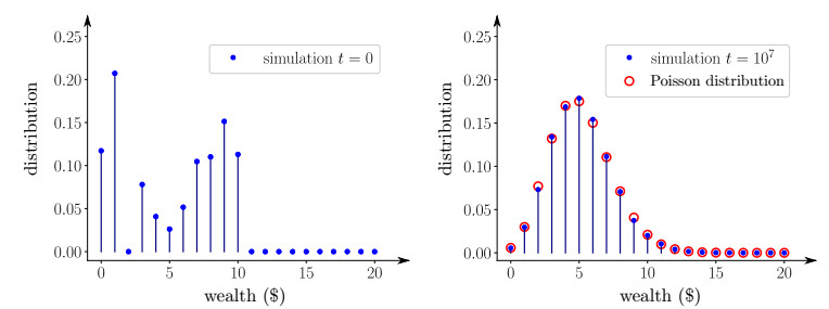
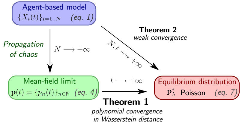
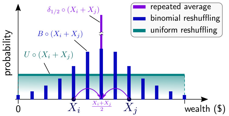
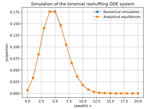
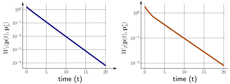
We present a novel reshuffling exchange model and investigate its long time behavior. In this model, two individuals are picked randomly, and their wealth $ X_i $ and $ X_j $ are redistributed by flipping a sequence of fair coins leading to a binomial distribution denoted $ B\circ (X_i+X_j) $. This dynamics can be considered as a natural variant of the so-called uniform reshuffling model in econophysics. May refer to Cao, Jabin and Motsch (2023), Dragulescu and Yakovenko (2000). As the number of individuals goes to infinity, we derive its mean-field limit, which links the stochastic dynamics to a deterministic infinite system of ordinary differential equations. Our aim of this work is then to prove (using a coupling argument) that the distribution of wealth converges to the Poisson distribution in the $ 2 $-Wasserstein metric. Numerical simulations illustrate the main result and suggest that the polynomial convergence decay might be further improved.
Citation: Fei Cao, Nicholas F. Marshall. From the binomial reshuffling model to Poisson distribution of money[J]. Networks and Heterogeneous Media, 2024, 19(1): 24-43. doi: 10.3934/nhm.2024002
We present a novel reshuffling exchange model and investigate its long time behavior. In this model, two individuals are picked randomly, and their wealth $ X_i $ and $ X_j $ are redistributed by flipping a sequence of fair coins leading to a binomial distribution denoted $ B\circ (X_i+X_j) $. This dynamics can be considered as a natural variant of the so-called uniform reshuffling model in econophysics. May refer to Cao, Jabin and Motsch (2023), Dragulescu and Yakovenko (2000). As the number of individuals goes to infinity, we derive its mean-field limit, which links the stochastic dynamics to a deterministic infinite system of ordinary differential equations. Our aim of this work is then to prove (using a coupling argument) that the distribution of wealth converges to the Poisson distribution in the $ 2 $-Wasserstein metric. Numerical simulations illustrate the main result and suggest that the polynomial convergence decay might be further improved.

| [1] |
F. Bassetti, G. Toscani, Mean field dynamics of interaction processes with duplication, loss and copy, Math. Models Methods Appl. Sci., 25 (2015), 1887–1925. https://doi.org/10.1142/S0218202515500487 doi: 10.1142/S0218202515500487

|
| [2] | F. Cao, S. Reed, A biased dollar exchange model involving bank and debt with discontinuous equilibrium, arXiv: 2311.07851, [Preprint], (2023) [cited 2024 Jan 08]. Available from: https://doi.org/10.48550/arXiv.2311.07851 |
| [3] |
F. Cao, S. Motsch, Derivation of wealth distributions from biased exchange of money, Kinet. Relat. Models, 16 (2023), 764–794. https://doi.org/10.3934/krm.2023007 doi: 10.3934/krm.2023007
|
| [4] |
F. Cao, PE. Jabin, S. Motsch, Entropy dissipation and propagation of chaos for the uniform reshuffling model, Math. Models Methods Appl. Sci., 33 (2023), 829–875. https://doi.org/10.1142/S0218202523500185 doi: 10.1142/S0218202523500185
|
| [5] |
F. Cao, Explicit decay rate for the Gini index in the repeated averaging model, Math. Methods Appl. Sci., 46 (2023), 3583–3596. https://doi.org/10.1002/mma.8711 doi: 10.1002/mma.8711
|
| [6] | F. Cao, PE. Jabin, From interacting agents to Boltzmann-Gibbs distribution of money, arXiv: 2208.05629, [Preprint], (2022) [cited 2024 Jan 08]. Available from: https://doi.org/10.48550/arXiv.2208.05629 |
| [7] |
F. Cao, S. Motsch, Uncovering a two-phase dynamics from a dollar exchange model with bank and debt, SIAM J. Appl. Math., 83 (2023), 1872–1891. https://doi.org/10.1137/22M1518621 doi: 10.1137/22M1518621
|
| [8] |
E. A. Carlen, E. Gabetta, G. Toscani, Propagation of smoothness and the rate of exponential convergence to equilibrium for a spatially homogeneous Maxwellian gas, Comm. Math. Phys., 199 (1999), 521–546. https://doi.org/10.1007/s002200050511 doi: 10.1007/s002200050511
|
| [9] | J. A. Carrillo, G. Toscani, Contractive probability metrics and asymptotic behavior of dissipative kinetic equations, Riv. Mat. Univ. Parma, 6 (2007), 75–198. https://ddd.uab.cat/record/44032 |
| [10] |
L P. Chaintron, A. Diez, Propagation of chaos: A review of models, methods and applications. I. Models and methods, Kinet. Relat. Models, 15 (2022), 895–1015. https://doi.org/10.3934/krm.2022017 doi: 10.3934/krm.2022017
|
| [11] |
A. Chakraborti, B. K. Chakrabarti, Statistical mechanics of money: how saving propensity affects its distribution, Eur. Phys. J. B, 17 (2000), 167–170. https://doi.org/10.1007/s100510070173 doi: 10.1007/s100510070173
|
| [12] |
A. Chatterjee, B. K. Chakrabarti, S. S. Manna, Pareto law in a kinetic model of market with random saving propensity, Physica A, 335 (2004), 155–163. https://doi.org/10.1016/j.physa.2003.11.014 doi: 10.1016/j.physa.2003.11.014
|
| [13] |
S. Chatterjee, P. Diaconis, A. Sly, L. Zhang, A phase transition for repeated averages, Ann. Probab., 50 (2022), 1–17. https://doi.org/10.1214/21-AOP1526 doi: 10.1214/21-AOP1526
|
| [14] |
R. Cortez, J. Fontbona, Quantitative propagation of chaos for generalized Kac particle systems, Ann. Appl. Probab., 26 (2016), 892–916. https://doi.org/10.1214/15-AAP1107 doi: 10.1214/15-AAP1107
|
| [15] | R. Cortez, Particle system approach to wealth redistribution, arXiv: 1809.05372, [Preprint], (2018) [cited 2024 Jan 08]. Available from: https://doi.org/10.48550/arXiv.1809.05372 |
| [16] | R. Cortez, F. Cao, Uniform propagation of chaos for a dollar exchange econophysics model, arXiv: 2212.08289, [Preprint], (2022) [cited 2024 Jan 08]. Available from: https://doi.org/10.48550/arXiv.2212.08289 |
| [17] | T. M. Cover, J.A. Thomas, Elements of information theory, John Wiley & Sons, 1999. https://doi.org/10.1002/0471200611 |
| [18] | G. Da Prato, An introduction to infinite-dimensional analysis, Springer Science & Business Media, 2006. https://doi.org/10.1007/3-540-29021-4 |
| [19] |
A. Dragulescu, V. M. Yakovenko, Statistical mechanics of money, Eur. Phys. J. B, 17 (2000), 723–729. https://doi.org/10.1007/s100510070114 doi: 10.1007/s100510070114
|
| [20] |
G. Gabetta, G. Toscani, B. Wennberg, Metrics for probability distributions and the trend to equilibrium for solutions of the Boltzmann equation, J. Stat. Phys., 81 (1995), 901–934. https://doi.org/10.1007/BF02179298 doi: 10.1007/BF02179298
|
| [21] |
B. T. Graham, Rate of relaxation for a mean-field zero-range process, Ann. Appl. Probab., 19 (2009), 497–520. 10.1214/08-AAP549 doi: 10.1214/08-AAP549
|
| [22] |
E. Heinsalu, P. Marco, Kinetic models of immediate exchange, Eur. Phys. J. B, 87 (2014), 1–10. https://doi.org/10.1140/epjb/e2014-50270-6 doi: 10.1140/epjb/e2014-50270-6
|
| [23] |
P E. Jabin, B. Niethammer, On the rate of convergence to equilibrium in the Becker–Döring equations, J Differ Equ, 191 (2003), 518–543. https://doi.org/10.1016/S0022-0396(03)00021-4 doi: 10.1016/S0022-0396(03)00021-4
|
| [24] |
N. Lanchier, Rigorous proof of the Boltzmann–Gibbs distribution of money on connected graphs, J. Stat. Phys., 167 (2017), 160–172. https://doi.org/10.1007/s10955-017-1744-8 doi: 10.1007/s10955-017-1744-8
|
| [25] |
N. Lanchier, S. Reed, Rigorous results for the distribution of money on connected graphs, J. Stat. Phys., 171 (2018), 727–743. https://doi.org/10.1007/s10955-018-2024-y doi: 10.1007/s10955-018-2024-y
|
| [26] |
N. Lanchier, S. Reed, Rigorous results for the distribution of money on connected graphs (models with debts), J. Stat. Phys., 176 (2019), 1115–1137. https://doi.org/10.1007/s10955-019-02334-z doi: 10.1007/s10955-019-02334-z
|
| [27] | T. M. Liggett, Interacting particle systems, New York: Springer, 1985. |
| [28] |
D. Matthes, G. Toscani, On steady distributions of kinetic models of conservative economies, J. Stat. Phys., 130 (2008), 1087–1117. https://doi.org/10.1007/s10955-007-9462-2 doi: 10.1007/s10955-007-9462-2
|
| [29] |
M. Merle, J. Salez, Cutoff for the mean-field zero-range process, Ann. Probab., 47 (2019), 3170–3201. https://doi.org/10.1214/19-AOP1336 doi: 10.1214/19-AOP1336
|
| [30] | G. Naldi, L. Pareschi, G. Toscani, Mathematical modeling of collective behavior in socio-economic and life sciences, Berlin: Springer Science & Business Media, 2010. https://doi.org/10.1007/978-0-8176-4946-3 |
| [31] |
G. Peyré, M. Cuturi, Computational optimal transport: With applications to data science, Found. Trends Mach. Learn., 11 (2019), 355–607. http://dx.doi.org/10.1561/2200000073 doi: 10.1561/2200000073
|
| [32] | R. Pymar, N. Rivera, Mixing of the symmetric beta-binomial splitting process on arbitrary graphs, arXiv: 2307.02406, [Preprint], (2023) [cited 2024 Jan 08]. Available from: https://doi.org/10.48550/arXiv.2307.02406 |
| [33] | A. Santos, Showing convergence of an infinite ODE system, MathOverflow 2022. Available from: https://mathoverflow.net/q/432268. |
| [34] | A S. Sznitman, Topics in propagation of chaos, in Ecole d'été de probabilités de Saint-Flour XIX—1989, Berlin: Springer, (1991), 165–251. https://doi.org/10.1007/BFb0085166 |
| [35] | R. Temam, Infinite-dimensional dynamical systems in mechanics and physics, Berlin: Springer Science & Business Media, 2012. https://doi.org/10.1007/978-1-4612-0645-3 |
Figures(5)
Fei Cao, Nicholas F. Marshall. From the binomial reshuffling model to Poisson distribution of money[J]. Networks and Heterogeneous Media, 2024, 19(1): 24-43. doi: 10.3934/nhm.2024002


 DownLoad: