Loading [MathJax]/jax/output/SVG/jax.js
Review Topical Sections

Seven Tesla MRI in Alzheimer's disease research: State of the art and future directions: A narrative review

  • Seven tesla magnetic resonance imaging (7T MRI) is known to offer a superior spatial resolution and a signal-to-noise ratio relative to any other non-invasive imaging technique and provides the possibility for neuroimaging researchers to observe disease-related structural changes, which were previously only apparent on post-mortem tissue analyses. Alzheimer's disease is a natural and widely used subject for this technology since the 7T MRI allows for the anticipation of disease progression, the evaluation of secondary prevention measures thought to modify the disease trajectory, and the identification of surrogate markers for treatment outcome. In this editorial, we discuss the various neuroimaging biomarkers for Alzheimer's disease that have been studied using 7T MRI, which include morphological alterations, molecular characterization of cerebral T2*-weighted hypointensities, the evaluation of cerebral microbleeds and microinfarcts, biochemical changes studied with MR spectroscopy, as well as some other approaches. Finally, we discuss the limitations of the 7T MRI regarding imaging Alzheimer's disease and we provide our outlook for the future.

    Citation: Arosh S. Perera Molligoda Arachchige, Anton Kristoffer Garner. Seven Tesla MRI in Alzheimer's disease research: State of the art and future directions: A narrative review[J]. AIMS Neuroscience, 2023, 10(4): 401-422. doi: 10.3934/Neuroscience.2023030

    Related Papers:

    [1] Cunjuan Dong, Changcheng Xiang, Wenjin Qin, Yi Yang . Global dynamics for a Filippov system with media effects. Mathematical Biosciences and Engineering, 2022, 19(3): 2835-2852. doi: 10.3934/mbe.2022130
    [2] Anji Yang, Baojun Song, Sanling Yuan . Noise-induced transitions in a non-smooth SIS epidemic model with media alert. Mathematical Biosciences and Engineering, 2021, 18(1): 745-763. doi: 10.3934/mbe.2021040
    [3] Dongmei Li, Bing Chai, Weihua Liu, Panpan Wen, Ruixue Zhang . Qualitative analysis of a class of SISM epidemic model influenced by media publicity. Mathematical Biosciences and Engineering, 2020, 17(5): 5727-5751. doi: 10.3934/mbe.2020308
    [4] Yanni Xiao, Tingting Zhao, Sanyi Tang . Dynamics of an infectious diseases with media/psychology induced non-smooth incidence. Mathematical Biosciences and Engineering, 2013, 10(2): 445-461. doi: 10.3934/mbe.2013.10.445
    [5] Toshikazu Kuniya, Hisashi Inaba . Hopf bifurcation in a chronological age-structured SIR epidemic model with age-dependent infectivity. Mathematical Biosciences and Engineering, 2023, 20(7): 13036-13060. doi: 10.3934/mbe.2023581
    [6] Jin Guo, Aili Wang, Weike Zhou, Yinjiao Gong, Stacey R. Smith? . Discrete epidemic modelling of COVID-19 transmission in Shaanxi Province with media reporting and imported cases. Mathematical Biosciences and Engineering, 2022, 19(2): 1388-1410. doi: 10.3934/mbe.2022064
    [7] Abdelheq Mezouaghi, Salih Djillali, Anwar Zeb, Kottakkaran Sooppy Nisar . Global proprieties of a delayed epidemic model with partial susceptible protection. Mathematical Biosciences and Engineering, 2022, 19(1): 209-224. doi: 10.3934/mbe.2022011
    [8] Yoichi Enatsu, Yukihiko Nakata, Yoshiaki Muroya . Global stability for a class of discrete SIR epidemic models. Mathematical Biosciences and Engineering, 2010, 7(2): 347-361. doi: 10.3934/mbe.2010.7.347
    [9] Yilei Tang, Dongmei Xiao, Weinian Zhang, Di Zhu . Dynamics of epidemic models with asymptomatic infection and seasonal succession. Mathematical Biosciences and Engineering, 2017, 14(5&6): 1407-1424. doi: 10.3934/mbe.2017073
    [10] Xinyu Liu, Zimeng Lv, Yuting Ding . Mathematical modeling and stability analysis of the time-delayed SAIM model for COVID-19 vaccination and media coverage. Mathematical Biosciences and Engineering, 2022, 19(6): 6296-6316. doi: 10.3934/mbe.2022294
  • Seven tesla magnetic resonance imaging (7T MRI) is known to offer a superior spatial resolution and a signal-to-noise ratio relative to any other non-invasive imaging technique and provides the possibility for neuroimaging researchers to observe disease-related structural changes, which were previously only apparent on post-mortem tissue analyses. Alzheimer's disease is a natural and widely used subject for this technology since the 7T MRI allows for the anticipation of disease progression, the evaluation of secondary prevention measures thought to modify the disease trajectory, and the identification of surrogate markers for treatment outcome. In this editorial, we discuss the various neuroimaging biomarkers for Alzheimer's disease that have been studied using 7T MRI, which include morphological alterations, molecular characterization of cerebral T2*-weighted hypointensities, the evaluation of cerebral microbleeds and microinfarcts, biochemical changes studied with MR spectroscopy, as well as some other approaches. Finally, we discuss the limitations of the 7T MRI regarding imaging Alzheimer's disease and we provide our outlook for the future.


    Abbreviations

    Aβ:

    beta-amyloid; 

    AD:

    Alzheimer's disease; 

    ASL:

    Arterial Spin Labelling; 

    BOLD:

    blood oxygenation level-dependent; 

    CA:

    Cornus Ammonis; 

    CA1-SRLM:

    stratum radiatum and lacunosum-moleculare of the Cornu Ammonis' field 1; 

    CBF:

    cerebral blood flow; 

    CEST:

    chemical exchange saturation transfer; 

    CMI:

    cerebral microinfarcts; 

    CNR:

    contrast-to-noise ratio; 

    CSF:

    cerebrospinal fluid; 

    DKI:

    diffusion kurtosis imaging; 

    DTI:

    diffusion tensor imaging; 

    EEG:

    electroencephalography; 

    FLAIR:

    fluid attenuated inversion recovery; 

    fMRI:

    functional MRI; 

    Gln:

    glutamine; 

    Glu:

    glutamate; 

    gluCEST:

    Chemical Exchange Saturation Transfer of glutamate; 

    GABA:

    γ-Aminobutyric acid; 

    GRE:

    gradient recalled echo; 

    LC:

    locus coeruleus; 

    MCI:

    mild cognitive impairment; 

    MI:

    myo-inositol; 

    MT:

    magnetization transfer; 

    MRS:

    MR Spectroscopy; 

    PET:

    Positron Emission Tomography; 

    PVS:

    perivascular spaces; 

    PiB:

    Pittsburgh compound B; 

    RF:

    radiofrequency; 

    SNR:

    signal-to-noise ratio; 

    SWI:

    susceptibility-weighted imaging; 

    TSE:

    turbo spin echo; 

    UHF:

    ultra-high field

    Infectious diseases have been a long-standing threat to human beings, claiming countless lives and causing catastrophic consequences for human survival and development. For instance, the Antonine plague in ancient Rome in 164 AD [1] resulted in numerous deaths, weakened the strength of ancient Rome to a certain extent and indirectly contributed to the decline of the Roman Empire. Similarly, the Black Death outbreaks in Europe between 1347–1353 [2] killed about one-third of the European population. The outbreak of SARS in 2003 [3] caused significant fatalities and economic losses. The H1N1 influenza virus that emerged in Mexico in 2009 [4] can cause pneumonia, leading to respiratory failure and multiple organ damage, resulting in death for some infected individuals. Moreover, the sudden onset of COVID-19 in 2020 [5,6,7,8] has had a profound impact on human health, the global economy and social behavior. These diseases have undoubtedly inflicted an incalculable toll on economic development and people's lives. Therefore, it is essential to investigate the spread of infectious diseases and propose effective prevention and control strategies. The study of infectious diseases has become crucial to address the long-standing problem of fulminant diseases that have plagued humanity. Since experimental research on infectious diseases is often challenging, appropriate mathematical models are frequently employed to reflect the transmission mechanism of diseases. The dynamic model of infectious disease is an effective approach commonly utilized in the theory and qualitative analysis of infectious disease [9]. By conducting qualitative and quantitative analyses of the model dynamics and numerical simulations, the critical factors affecting the spread of infectious diseases can be identified and the future development trend can be predicted. This provides strong theoretical and data support for the prevention and control of infectious diseases, enabling accurate and effective disease prevention.

    The spread of infectious diseases is influenced by numerous factors, including media reports [10,11,12,13,14,15], population density [16] and vaccination [17]. In modern times, the media plays a significant role in shaping people's lifestyles, and its impact on the spread of infectious diseases is crucial. During an epidemic of infectious diseases, people often rely on the media, including news and broadcasts, to share information about disease prevention, control and their own experiences in fighting the disease. The media reports the spread of diseases promptly and through various channels, and people take appropriate measures, such as wearing masks, maintaining personal hygiene, reducing visits to public places and frequently washing their hands, to prevent and reduce the spread and occurrence of diseases [18]. Thus, it is practical to consider the influence of media factors in the infectious disease model and to optimize the control strategy of infectious diseases to obtain reasonable prevention and control measures.

    There are various types of infectious disease models that can be influenced by media reports, such as continuous models, switched models and discrete models. However, researchers typically opt to use continuous models to study the influence of media coverage on disease transmission. In 2007, Liu et al. [19] conducted pioneering research on the influence of media and psychological effects on infectious diseases. They proposed a continuous infectious disease model with an infectious rate of βea1Ea2Ia3H. In 2008, Cui et al. [20] introduced a media influence function of βemI and developed a continuous SEI model. The variable m represents the psychological reaction of the public after learning about the disease through media reports. The dynamic behavior of the model was analyzed with varying values of m to evaluate the influence of media on the spread and control of the disease. Furthermore, switching models have also been studied by many researchers, in combination with other factors. A switching system is generally composed of some subsystems and a switching signal [21,22]. Its main feature is that the rich dynamic behavior of the original system becomes more complicated under the action of the switching signal. In 2013, Xiao et al. [23] established a continuous infectious disease model with a media impact factor M(I,dI/dt), and studied the role of the media and behavioral changes of consciousness by considering the existence of a threshold for susceptibles. They then transformed the model into a switching system and concluded that media or psychological influence will delay the peak of the epidemic and cause a small-scale disease outbreak. Liu et al. [24] established a SIR epidemic model having a non-smooth function f(I) and analyzed the dynamics of the infectious disease switching system through a saturation function to explore the impact of media reports on the spread of infectious diseases. Zhao [25] considered the media impact factor function β(I)=β/(1+εmI) to establish a Filippov model with a media switching threshold strategy. They concluded that the greater the media's propaganda, the more beneficial the disease control and elimination.

    The aforementioned work is based on research and analysis conducted using either a continuous model or a continuous switching model. When the population size is large, the changes in the number of susceptible and infected individuals can be approximated as continuous over time, making it reasonable to use a continuous model. However, when the spread of infectious diseases is slow, or data collection occurs on a yearly, monthly, weekly or daily basis, population changes occur discretely rather than continuously. Therefore, using discrete models to describe the dynamic behavior of infectious diseases is more appropriate in such situations. These models can also provide more effective and accurate data references for subsequent disease prevention and control measures.

    Compared to continuous infectious disease models, there are fewer studies on discrete infectious disease models [26,27]. Moreover, there are even fewer studies on discrete switching infectious disease models that take into account the influence of media reports. In this study, we will focus on the discrete infectious disease switching model that incorporates a media influence factor of βemI. To better reflect real-world scenarios, we consider a switching model that includes the economic threshold (ET) [28,29] of infected individuals. We explore the dynamic behavior of the system when the number of infected individuals exceeds the critical ET. The objective is to investigate the impact of media reports on the epidemic trend of infectious diseases, analyze the dynamic behaviors arising from influential factors and provide effective strategies for prevention and control of infectious disease to keep the number of infected individuals within a desired threshold level.

    The rest of the paper is structured as follows. In the next section, we propose a non-smooth infectious disease switching model that can effectively capture the influence of media reports. In Section 3, we provide a qualitative analysis of the two subsystems. Section 4 is devoted to numerical simulations to explore the impact of initial population density on disease outbreaks and to analyze the bifurcation of sensitive parameters. Finally, we conclude the paper with a discussion of our findings and their implications for infectious disease prevention and control measures in the last section.

    Kermack and McKendrick introduced the SIR compartment model [30] in 1927, which has become a popular tool for studying infectious diseases. One of its key assumptions is that individuals who recover from the disease will develop lifelong immunity, as seen in diseases such as chickenpox and measles. Building on this, the SIR continuous model can be formulated by the following equation set:

    {S(t)=ΛβS(t)I(t)μS(t),I(t)=βS(t)I(t)(μ+δ+γ)I(t),R(t)=γS(t)μR(t), (2.1)

    where S(t),I(t) and R(t) respectively represent the number of susceptibles, infected individuals and recoveries at time t; Λ is the recruitment rate of the individuals at a time, β is infection rate, μ is the natural death rate, δ is the mortality rate due to disease and γ is the recovery rate from infection.

    Due to the discontinuity of data collection units and changes in population, we adopt a discrete-time infectious disease model to better reflect the actual situation. There are several approaches to building a discrete model, but the most commonly used method is to discretize a continuous model. The two commonly used methods are the Mickens non-standard discrete method and the Euler discrete method. Motivated by [31,32,33], the Euler method was used to discretize the model (2.1). The resulting discrete model is shown below:

    {Sn+1=Sn+ΛβSnInμSn,In+1=In+βSnIn(μ+δ+γ)In,Rn+1=Rn+γInμRn. (2.2)

    Based on model (2.2), we now incorporate the effect of media influence factor m by modifying the infection rate β to βemI. The updated model is expressed as follows

    {Sn+1=Sn+ΛβemISnInμSn,In+1=In+βemISnIn(μ+δ+γ)In,Rn+1=Rn+γSnInμRn. (2.3)

    Typically, there is no media coverage when the quantity of infected individuals is small and does not exceed the ET. In such cases, the disease fails to capture the attention of the public at large. However, once the number of infected individuals abruptly surges and surpasses the ET, the role of media influence becomes significant. Media reports and publicity can draw the public's attention towards the disease dynamics and prompt individuals to alter their behavior and take appropriate protective measures.

    Taking advantage of the threshold policy, we combine models (2.2) and (2.3) as follows

    {Sn+1=Sn+ΛβSnInμSn,In+1=In+βSnIn(μ+δ+γ)In,Rn+1=Rn+γInμRn,}In<ET,Sn+1=Sn+ΛβemISnInμSn,In+1=In+βemISnIn(μ+δ+γ)In,Rn+1=Rn+γInμRn,}InET. (2.4)

    Note that the first two equations of models (2.2) and (2.3) do not involve the variable R. To simplify model (2.4), we can express it as

    {Sn+1=Sn+ΛβSnInμSn,In+1=In+βSnIn(μ+δ+γ)In,}In<ET,Sn+1=Sn+ΛβemISnInμSn,In+1=In+βemISnIn(μ+δ+γ)In,}InET. (2.5)

    The discrete switching model (2.5) expresses a dynamic system that adheres to a threshold policy, whereby media influence is only effective when InET. For more information on the threshold policy, please refer to [28,29]. Similar modeling approaches can also be found in the literature, such as in references [34,35].

    The two subsystems of discrete switching model (2.5) are qualitatively analyzed, including existence and stability, to explore the complex dynamic behavior of the model in this section.

    Denoting F(Z)=InET with vector Z=(Sn,In)T, and

    SG1(Z)=[Sn+ΛβSnInμSnIn+βSnIn(μ+δ+γ)In], (3.1)
    SG2(Z)=[Sn+ΛβemISnInμSnIn+βemISnIn(μ+δ+γ)In], (3.2)

    so switching system (2.5) can be rewritten as a vector

    Z(t)={SG1(Z),ZG1,SG2(Z),ZG2, (3.3)

    where

    G1={ZR2+:F(Z)<0,Sn>0,In>0,}. (3.4)
    G2={ZR2+:F(Z)0,Sn>0,In>0.}. (3.5)

    Using the threshold policy, we define regions G1 and G2 of system (3.3) as SG1 and SG2, respectively. Subsequently, we will investigate the dynamical behavior of subsystems SG1 and SG2. Below, we present the definition of regular equilibria for switching systems, which will be utilized in this paper [36].

    Definition 3.1. A real (virtual) equilibrium Z=(SG,IG) for system (3.3) is defined as follows: if Z is an equilibrium for subsystem SG1 and F(Z)<0 (F(Z)0), or if Z is an equilibrium for subsystem SG2 and F(Z)0 (F(Z)<0). Denoted the real (virtual) equilibrium Z by ErGi (EvGi) for subsystem SGi, respectively. The real and virtual equilibria are all named regular equilibria.

    Given the biological significance of system (3.3), it is crucial to establish the existence of positive invariant sets for subsystem SG1 to ensure the non-negativity of the system's solution.

    Lemma 3.1. The bounded set

    Ω1={(SG1n,IG1n)|SG1n>max{0,μ+δ+γ1β},  Λ>(μ1+βIG1n)SG1n}

    is a positive invariant set of subsystem SG1.

    Proof. As n=0, it follows from (3.1) and (3.4) that

    {SG11=Λ+(1βIG10μ)SG10,IG11=IG10[1+βSG10(μ+δ+γ)], (3.6)

    and SG10>0,IG10>0. In order to prove SG11>0, it has got to prove

    Λ>(μ1+βIG10)SG10,

    and this is our hypothesis.

    To prove IG11>0, it is obtained from the second formula of (3.6) that

    1+βSG10(μ+δ+γ)>0,

    i.e.,

    SG10>μ+δ+γ1β.

    It is important to establish the relationship between 0 and μ+δ+γ1β, so we obtain that

    SG10>max{0,μ+δ+γ1β}.

    Analogically, when n=k, if the conditions SG1k>max{0,μ+δ+γ1β},  Λ>(μ1+βIG1k)SG1k hold true, then we have SG1k+1>0,IG1k+1>0.

    Hence, Ω1 is the positive invariant set of SG1. The proof is completed.

    The equilibrium of system SG1 is determined by the following equations

    {ΛβSnInμSn=0,βSnIn(μ+δ+γ)In=0. (3.7)

    Therefore, there is a disease-free equilibrium P1=(Λ/μ,0). Let us define the basic reproduction number as RG10=βΛ/[μ(μ+δ+γ)]. Consequently, we can obtain the unique positive equilibrium

    EG1=(SG1,IG1)=(μ+δ+γβ,Λμ+δ+γμβ)=(ΛμRG10,μ(RG101)β).

    This completes the proof.

    Next, we will explore the local stability of the positive equilibrium(SG1,IG1).

    Theorem 3.2. The positive equilibrium EG1=(SG1,IG1) of system SG1 is asymptotically stable, provided that

    max{1,μ(μ+δ+γ)4μ(μ+δ+γ)2μ}<RG10<μ+δ+γ1+μ+δ+γ, (3.8)

    where

    (μ+δ+γ)>max{2,4μ}.

    Proof.

    The Jacobian Matrix J1 of the equilibrium EG1=(SG1,IG1) is

    J1=[1μβIG1βSG1βIG1βSG1+1(μ+δ+γ)].

    From Eq (3.7), we can acquire the characteristic equation for the Jacobian matrix J1 of system SG1 at (SG1,IG1), and the characteristic equation is

    P(λ)=λ2(trJ1)λ+detJ1 (3.9)

    and

    P(1)=1trJ1+detJ1=μ(RG101)(μ+δ+γ),
    P(1)=1+trJ1+detJ1=42μRG10+μ(RG101)(μ+δ+γ).

    Condition (3.8) ensures that inequalities

    detJ1<1,P(1)>0,P(1)>0

    hold. Using the Jury et al. [37], we can demonstrate that the modulus of all the roots of Eq (3.9) is less than 1, and the endemic equilibrium EG1=(SG1,IG1) is locally asymptotically stable.

    Similar to subsystem SG1, and considering the biological significance of the model, its solution must not be negative. Therefore, we have first derived the following results.

    Lemma 3.3. The bounded set

    Ω2={(SG2n,IG2n)|emIG2nSG2n>max{0,μ+δ+γ1β}, Λ>(μ1+βemIG2nIG2n)SG2n}

    is a positive invariant set of subsystem SG2.

    Since the proof method is similar to Lemma 3.1, we have omitted the proof process.

    The equilibrium of system SG2 is determined by the following equations

    {ΛβemInSnInμSn=0,βemInSnIn(μ+δ+γ)In=0. (3.10)

    Obviously, system SG2 exists a disease free equilibrium P2=(Λ/μ,0), and the endemic equilibrium EG2=(SG2,IG2) satisfies

    Λ(μ+δ+γ)IG2μ(μ+δ+γ)emIG2β=0.

    Defining x=IG2, then

    f(x)=aemx+bx+c=0, (3.11)

    where

    a=μ(μ+δ+γ)β>0,b=(μ+δ+γ)>0,c=Λ<0.

    In addition, we study the positive equilibrium (SG2,IG2) of SG2 by numerical methods. It follows from Eq (3.10) that

    Λ(μ+δ+γ)IG2=μ(μ+δ+γ)emIG2β. (3.12)

    Defining two auxiliary functions

    {F(x)=Λ(μ+δ+γ)xG(x)=μ(μ+δ+γ)emIG2β (3.13)

    to verify the existence of an equilibrium for system SG2, Figure 1 shows F(x) and G(x) under different β. As F(0)>G(0), two functions always intersect at a point, indicating the existence of the equilibrium for subsystem SG2. The existence of an equilibrium in system SG2 has been established, and its stability is now being investigated.

    Figure 1.  The existence of the equilibrium (SG2,IG2) of the subsystem SG2, parameters are Λ=1,γ=0.5,δ=0.02,μ=0.2,m=3.

    Theorem 3.4. The positive equilibrium of system SG2, denoted by EG2=(SG2,IG2), is asymptotically stable provided that

    {ΛβemIG2>μ(μ+δ+γ)(1mIG2),(12μ+δ+γ)ΛβemIG2>4+μ(μ+δ+γ)+(2μ)(μ+δ+γ)mIG2,(11μ+δ+γ)ΛβemIG2<μ(μ+δ+γ)+(1μ)(μ+δ+γ)mIG2. (3.14)

    Proof. For the positive equilibrium (SG2,IG2) of the system SG2, we can get the characteristic equation of the Jacobian matrix J2 for the subsystem SG2 evaluated at (SG2,IG2).

    P(λ)=λ2(trJ2)λ+detJ2 (3.15)

    and

    J2=[1μβemIG2IG2βSG2emIG2(1mIG2)βemIG2IG2βSG2emIG2(1mIG2)+1(μ+δ+γ)].

    Clearly,

    trJ2=21μ+δ+γΛβemIG2(μ+δ+γ))mIG2,
    detJ2=1+(μ1)(μ+δ+γ)mIG2+(11μ+δ+γ)ΛβemIG2μ(μ+δ+γ).

    According to the Jury et al. [37], the condition for the local stability of the equilibrium EG2 is

    |trJ2|<detJ2+1<2. (3.16)

    Conditions (3.14) guarantee the validity of the inequality (3.16), which implies that the endemic disease equilibrium (SG2,IG2) of subsystem SG2 is locally asymptotically stable.

    In this section, we will study the complex dynamics of the infectious disease switching system (3.3). This is a complex, nonlinear dynamic system with a threshold strategy, making it difficult to analyze in detail theoretically. Therefore, we will analyze the bifurcation [38,39,40] of parameters and the outbreak state under the influence of initial density by numerical simulations.

    Based on Definition 3.1, this section mainly focuses on the real and virtual equilibrium states of the two subsystems in system (3.3) and conducts a dynamic behavior analysis on them through numerical simulations. To clearly demonstrate the existence of various equilibrium parameter spaces, we have selected γ and ET as bifurcation parameters while fixing other parameters, as shown in Figure 2. Observing the parameter space plane when ET ranges from 0 to 6 and γ ranges from 0 to 1, it is divided into five regions. When the recovery rate γ is within the range of [0,0.325][0.725,1], two regions can be identified: region Ⅰ-1 only has the existence of ErG1, while region Ⅰ-2 only has the existence of EvG1. In the case of intermediate recovery rates (γ[0.325,0.725]), it can be observed that ErG1 and ErG2 coexist in Ⅱ-1, EvG1 and ErG2 coexist in Ⅱ-2, and EvG1 and EvG2 coexist in Ⅱ-3. Figure 2 displays various bifurcaiton phenomena, which provide important insights into how to hold back the disease outbreaks or control the density of infected individuals in areas below the threshold ET. Through numerical analysis, we can select an appropriate threshold ET such that the equilibrium state of subsystem SG2 is a virtual equilibrium state, which can help us achieve our control objectives.

    Figure 2.  Bifurcation diagram for the existence of equilibria of model (3.3) to γ and ET, other parameters are Λ=1.8,m=0.4,β=0.06,μ=0.05,δ=0.05.

    Codimension-1 bifurcation analysis is a common method to obtain a preliminary understanding of dynamic behavior. It provides information about the influence of a specific parameter on dynamics. We analyze the codimension one bifurcation diagrams of the parameters μ, δ, and β separately to observe the type of attractor and its change with the variation of the parameter.

    First, we select μ as the bifurcation parameter to study the complex dynamic behavior of system (3.3) while fixing other parameters as shown in Figure 3. When μ increases from 0.863 to 0.902, periodic solutions, chaotic solutions, and periodic doubling solutions can be observed. Further, as the parameter μ changes from 0.8656 to 0.8783, the solution of system (3.3) becomes stable. Notably, at μ=(0.8827,0.8958), the system exhibits an obvious chaotic state. The bifurcation diagram illustrates that small perturbations in parameters can lead to significant changes in the system's dynamic behavior.

    Figure 3.  Bifurcation diagram for model (3.3) concerning μ. All other parameters are as follows: Λ=0.9,ET=1,m=0.04,β=0.0009,δ=1.187,γ=0.1.

    Second, building upon the bifurcation Figure 3, we held other parameters constant and explored various states of the system's solutions by selecting different values of δ, as shown in Figure 4. When δ=1.18 in Figure 4 (A), system (3.3) has a stable solution. However, when δ increases from 1.18 to 1.2, the system exhibits a periodic solution, as shown in Figure 4(B). As δ reaches 1.22 or 1.252, a chaotic solution abruptly emerges, as depicted in Figure 4 (C), (D). As the parameter continues to change, the nature of the system's solutions undergoes fundamental shifts, highlighting the significant influence of parameters on the system.

    Figure 4.  Phase-plan of model (3.3) with different δ. All other parameters are as follows: Λ=0.9,ET=1,m=0.01,β=0.004,μ=0.81,γ=0.1, and [A] δ=1.18, [B] δ=1.2, [C] δ=1.22, [D] δ=1.252.

    Third, we investigate β in the system as the bifurcation parameter, while keeping other parameters unchanged. Figure 5 exhibitions that the system exhibits very complex dynamic behaviors when β increases. In particular, in the interval of β(0,1.6), the system displays period-doubling branches, chaotic solutions and periodic solutions. In Figure 5, the system (3.3) exhibits multiple periodic and chaotic solutions, such as for β[0.04,0.652][0.99,1.45]. This highlights the available impact of the infection rate on disease transmission.

    Figure 5.  Bifurcation diagram for model (3.3) concerning β. All other parameters are as follows: Λ=10,μ=0.049,ET=3,γ=0.9,δ=0.04,m=0.7.

    To further understand the influence of parameter μ on the system in this state, we explore values between 0.01 and 0.6, as shown in Figure 6, and observe that different natural mortality rates can affect the system's dynamic behavior. The bifurcation diagrams of system (3.3) with respect to β under the influence of μ become increasingly simpler, as depicted in Figures 6 (A)(C).

    Figure 6.  Bifurcation diagram for model (3.3) concerning β. All other parameters are as follows: Λ=10,ET=9,m=0.7,δ=0.03,γ=0.43, and [A] μ=0.001, [B] μ=0.01, [C] μ=0.1.

    In addition to the significant and sensitive parameters that have a crucial impact on disease transmission, the initial density of susceptible and infected individuals in a given area can also have varying effects on the outbreak state of the disease. This section systematically investigates the dynamic behavior of the switching system (3.3) under different initial conditions.

    To investigate the interaction between initial density and media factors, we fix the parameter values as shown in Figure 7 and analyze the different scenarios presented by different initial densities. In Figure 7(A), with an initial density of (13, 1.7), the numerical simulation results show that the density of infected individuals never exceeds the given ET=2, indicating that media factors are not required to control the outbreak.

    Figure 7.  Switching impact of model (3.3) under different initial densities. All other parameters are as follows: Λ=12,ET=2.5,m=0.09,μ=0.55,δ=1.25,γ=0.3, and [A] (S0,I0)=(13,1.7), [B] (S0,I0)=(12,1.5), [C] (S0,I0)=(11.7,2), [D] (S0,I0)=(11,1).

    However, for initial densities of (12, 1.5) or (11.7, 2), the results indicate that the system will be affected by media factors once or twice, and the density of infected individuals will stabilize in the system area, as shown in Figure 7(B), (C). On the other hand, when the initial density is (11, 1), society must strengthen public's attention and protective measures through the influence of media factors multiple times to keep the density of infected individuals below ET.

    Furthermore, we analyzed the effect of the initial population density on the outbreak of infectious diseases by creating a horizontal classification map of susceptibles and infected individuals while keeping other parameters fixed (see Figure 7). As shown in Figure 8, infectious diseases will not break out in region Ⅰ, and the impact of media reports on the population is minimal since the disease is not serious. In green zone Ⅱ, an outbreak will occur when the initial population density is within a certain range. As the number of infected people exceeds the threshold, media coverage will play a role in preventing susceptible groups from being infected and controlling the spread of infectious diseases. There will be two outbreaks in area Ⅲ, and the media needs to repeatedly emphasize and remind everyone to pay attention to it. Eventually, there will be no further outbreaks. The solution of the system in area Ⅳ will not be affected by media factors after three outbreaks, while the solution in area Ⅴ will experience more than three outbreaks. Clearly, when the number of infected people exceeds ET, different initial population densities within a certain range will lead to varying outbreak frequencies of infectious diseases. Similarly, when we vary the values of other parameters, we can also observe similar phenomena, as shown in Figure 9.

    Figure 8.  The frequency of disease outbreaks at the initial density (S0,I0) of the system (3.3). All other parameters are as follows: Λ=12,ET=2.5,μ=0.55,δ=1.25,γ=0.3,m=0.09,β=0.15.
    Figure 9.  The frequency of disease outbreaks at the initial density (S0,I0) of the system (3.3). All other parameters are as follows: Λ=1.7,ET=2,μ=0.05,δ=1.2,γ=0.3,m=0.11,β=0.15.

    Based on the above analysis, it can be inferred that the initial population density plays a crucial role in disease outbreaks, and monitoring population density in endemic areas can be beneficial for preventing and controlling infectious diseases.

    As previously mentioned, the switching system for infectious diseases reveals various dynamic behaviors, including the coexistence of multiple attractors. To better understand its biological significance, we selected different initial densities while fixing other parameters, as shown in Figure 10.

    Figure 10.  Coexisting attractors of model (3.3) with different initial values. All other parameters are as follows: Λ=16,ET=2,β=0.3,μ=0.8,δ=1,γ=0.1; [A] (S0,I0)=(7.9,1.91), [B] (S0,I0)=(9,1.8).

    For instance, when m=0.066, two infectious disease outbreak attractors exist simultaneously, exhibiting different outbreak frequencies and amplitudes (i.e., Figure 10(A), (B). On one hand, if the initial values (S0,I0) are set to (7.9,1.91), the attractor exhibits the amplitude and frequency shown in Figure 10(A), which is approximated by the solution of system (3.3). On the other hand, when the initial values (S0,I0) change to (9,1.8), the amplitudes and frequencies become different from those in Figure 10(A), displaying a more complex burst pattern, as shown in Figure 10(B).

    Figure 11 illustrates three periodic outbreak attractors with different amplitudes and periods, which are selected by fixing three population inputs. If we fix the initial population density as (100,10), the three attractors coexist and exhibit different amplitudes and frequencies with different values of population inputs. Corresponding to Λ=130,150,300, we can observe that the three attractors have different periods of 3, 6 and 5, respectively. In particular, the periodic attractor in the third condition has the largest amplitude for both susceptible and infected persons, and the outbreak pattern is the most complex. In the first case, the outbreak pattern is similar to that in the second case, but the outbreak cycle is very different.

    Figure 11.  Coexisting attractors of model (3.3) with different Λ. All other parameters are as follows: (S0,I0)=(100,10),ET=15,m=0.1,β=2.8,μ=0.18,γ=0.12,δ=0.1; [A, B] Λ=130, [C, D] Λ=150, [E, F] Λ=300.

    Based on the analysis of attractors in Figures 10 and 11, it is evident that the initial densities and population inputs of susceptible and infected individuals may lead to different intervention strategies for controlling the outbreak of an epidemic. Therefore, in addition to monitoring population density in endemic areas, it is also necessary to consider population movements.

    Furthermore, the initial density also impacts the switching frequency of the infectious disease switching system (3.3), as depicted in Figure 12 (A)(C). Notably, Figure 12 (A)(C) underwent 13 and 15 switching events, respectively. Figure 12 (D)(F) illustrate the correlation between switching time and frequency corresponding to Figure 12 (A)(C), respectively.

    Figure 12.  Switching frequency (S–F) and switching time (S–T) of system (3.3). Parameters are ET=10,m=0.1,β=0.3,μ=0.8,γ=0.1,δ=1,Λ=15. The initial densities from top to bottom are (3.88, 7.95), (4.61, 5.47) and (7.25, 4.71).

    The switching frequency in Figure 12 (D) initially stabilized at 5, subsequently fluctuating within the range of [4,9], but with an overall increasing trend. The switching frequency in Figure 12 (E) remained at 5 during the fourth switching and decreased to 4 during the final switching. The switching frequency in Figure 12 (F) also stabilized at 5 and then rose to 9 during the last switching event. Elevated system switching occurrences imply a need for more frequent implementation of control measures. This, in turn, indirectly escalates media coverage frequency and the associated reporting costs. Consequently, accounting for the initial value becomes imperative when devising strategies for managing infectious diseases.

    In this paper, we research the dynamics model of infectious disease affected by media reports and the threshold of infected persons. We derived and established a discrete switching infectious disease model and performed a qualitative analysis of its subsystem. The dynamic behavior of the model was analyzed using various methods, including codimension two bifurcation diagrams, codimension one bifurcation diagrams and initial sensitivity. We found that multiple parameters and population density in an area can influence infectious disease outbreaks under the influence of vectors, providing important information for the eradication of infectious diseases. Our results highlight the need to consider media reports and population movements when monitoring and controlling infectious diseases. To explore the dynamic behavior of the model, we employ qualitative analysis techniques related to differential equations to study the existence and stability of equilibria in the subsystems. Using codimension two bifurcation analysis, we identify regions where the system has true and false equilibria, as shown in Figure 2. Based on these findings, a reasonable threshold ET can be designed for preventing and treating infectious diseases to maintain a stable true equilibrium in system (3.1) and a virtual equilibrium in system (3.2), thereby promoting disease eradication.

    Since various parameters can potentially affect the dynamic behavior of the system, we analyzed the possible bifurcation behavior of system (3.3) as shown in Figures 36, which exhibits a variety of dynamic behaviors such as periodic and chaotic solutions, multistability and period doubling bifurcations. The branching diagram reveals that the path to chaos is very intricate, demonstrating that hidden factors such as infection rate, natural mortality, mortality due to disease, etc., affect the dynamic behavior of the system. The media reports influence factor m indirectly affects the changes in these factors. This illustrates that people's influence through media reports can increase awareness of prevention and lead to corresponding preventive and control measures, thereby reducing the spread of diseases. Furthermore, we also explored the relationship between the initial population density and the prevention of infectious diseases. Figures 79 provide evidence that changes in population density, under the influence of media reports, can cause different disease outbreaks through the codimension two bifurcation map and the codimension one bifurcation map. Furthermore, Figure 10 shows that different population densities, when the fixed m remains unchanged, will produce different attractors and the complexity of system dynamics will also differ. The coexistence of three attractors in Figure 11 also reflects that different population inputs lead to similar phenomena. Therefore, reasonable and effective monitoring and control of population densities and inputs in epidemic areas, under the influence of the media, is conducive to prevent and control the infectious diseases.

    Moreover, we have presented the switching frequency and switching time of the system (3.3) under various initial conditions, highlighting the relationship between initial density and the control of infectious diseases. The results demonstrate that the initial density of susceptible and infected individuals influences the ultimate state following the onset of infectious diseases, as illustrated in Figure 12. The variability in switching frequencies further reinforces this observation. Hence, incorporating the initial value becomes a significant aspect in the study of infectious disease switching systems.

    We have investigated the dynamic behavior of the infectious disease switching system under the influence of media coverage. However, the limitation of medical resources also affects the speed and efficiency of disease control. If the maximum hospital capacity is significantly lower than the threshold of media response, it would be crucial to incorporate the resource limitation into the infectious disease switching model. This is an important topic for future research both theoretically and practically. Furthermore, for comparative analysis, regarding the continuous counterpart of the discrete switching infectious disease model, we will employ the Filippov switching model to depict it. We will provide corresponding comparative studies as well. This is a meaningful topic that deserves further in-depth investigation.

    The author declares that no AI tools were utilized for data analysis, modeling, or decision-making processes.

    This work is supported by National Natural Science Foundation of China (No. 12261104, 12361104), and the Youth Talent Program of Xingdian Talent Support Plan (XDYC-QNRC-2022-0708).


    Conflicts of interest


    The authors have no conflicts of interest to declare.

    [1] Masters CL, Bateman R, Blennow K, et al. (2015) Alzheimer's disease. Nat Rev Dis Primers 1. https://doi.org/10.1038/nrdp.2015.56
    [2] Prince M, Bryce R, Albanese E, et al. (2013) The global prevalence of dementia: a systematic review and meta-analysis. Alzheimers Dement 9: 63-75.e2. https://doi.org/10.1016/j.jalz.2012.11.007
    [3] 
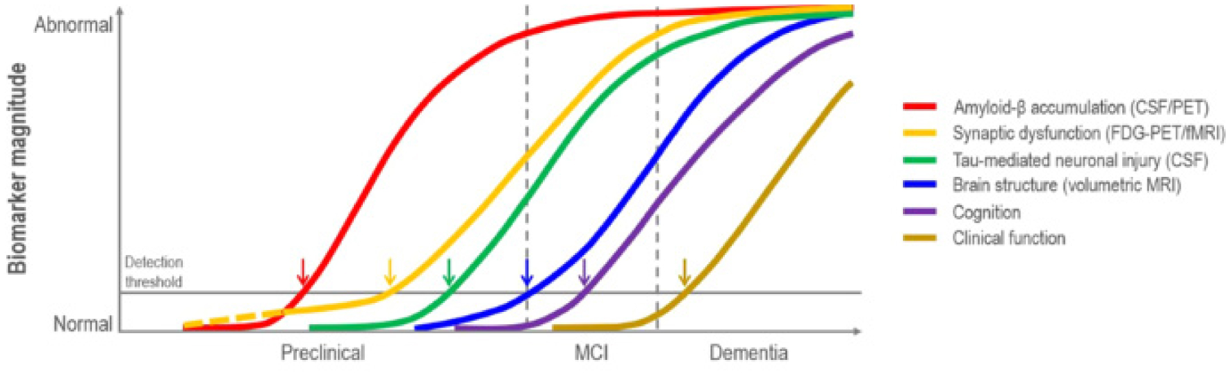
Jack CR, Knopman DS, Jagust WJ, et al. (2010) Hypothetical model of dynamic biomarkers of the Alzheimer's pathological cascade. Lancet Neurol 9: 119-128. https://doi.org/10.1016/S1474-4422(09)70299-6
    [4] Lee BC, Mintun M, Buckner RL, et al. (2003) Imaging of Alzheimer's disease. J Neuroimaging 13: 199-214. https://doi.org/10.1111/j.1552-6569.2003.tb00179.x
    [5] McKhann GM, Knopman DS, Chertkow H, et al. (2011) The diagnosis of dementia due to Alzheimer's disease: recommendations from the National Institute on Aging-Alzheimer's Association workgroups on diagnostic guidelines for Alzheimer's disease. Alzheimers Dement 7: 263-269. https://doi.org/10.1016/j.jalz.2011.03.005
    [6] Knopman DS, Amieva H, Petersen RC, et al. (2021) Alzheimer disease. Nat Rev Dis Primers 7: 33. https://doi.org/10.1038/s41572-021-00269-y
    [7] Arachchige ASPM (2022) 7-Tesla PET/MRI: A promising tool for multimodal brain imaging?. AIMS Neurosci 9: 516-518. https://doi.org/10.3934/Neuroscience.2022029
    [8] Okada T, Fujimoto K, Fushimi Y, et al. (2022) Neuroimaging at 7 Tesla: a pictorial narrative review. Quant Imag Med Surg 12: 3406-3435. https://doi.org/10.21037/qims-21-969
    [9] Zwanenburg JJ, van der Kolk AG, Luijten PR (2013) Ultra-High-Field MR Imaging: Research Tool or Clinical Need?. PET Clin 8: 311-328. https://doi.org/10.1016/j.cpet.2013.03.004
    [10] Apostolova LG, Zarow C, Biado K (2015) Relationship between hippocampal atrophy and neuropathology markers: a 7T MRI validation study of the EADC-ADNI Harmonized Hippocampal Segmentation Protocol. Alzheimers Dement 11: 139-150. https://doi.org/10.1016/j.jalz.2015.01.00
    [11] Düzel E, Costagli M, Donatelli G, et al. (2021) Studying Alzheimer disease, Parkinson disease, and amyotrophic lateral sclerosis with 7-T magnetic resonance. Eur Radiol Exp 5. https://doi.org/10.1186/s41747-021-00221-5
    [12] Theysohn JM, Kraff O, Maderwald S, et al. (2009) The human hippocampus at 7 T--in vivo MRI. Hippocampus 19: 1-7. https://doi.org/10.1002/hipo.20487
    [13] Kerchner GA, Hess CP, Hammond-Rosenbluth KE, et al. (2010) Hippocampal CA1 apical neuropil atrophy in mild Alzheimer disease visualized with 7-T MRI. Neurology 75: 1381-1387. https://doi.org/10.1212/WNL.0b013e3181f736a1
    [14] Barazany D, Assaf Y (2012) Visualization of cortical lamination patterns with magnetic resonance imaging. Cereb Cortex 22: 2016-2023. https://doi.org/10.1093/cercor/bhr277
    [15] Deng M, Yu R, Wang L, et al. (2016) Learning-based 3T brain MRI segmentation with guidance from 7T MRI labeling. Med Phys 43. https://doi.org/10.1118/1.4967487
    [16] Cheng PW, Chiueh TD, Chen JH (2021) A high temporal/spatial resolution neuro-architecture study of rodent brain by wideband echo planar imaging. Sci Rep 11. https://doi.org/10.1038/s41598-021-98132-3
    [17] Yoo PE, John SE, Farquharson S, et al. (2018) 7T-fMRI: Faster temporal resolution yields optimal BOLD sensitivity for functional network imaging specifically at high spatial resolution. NeuroImage 164: 214-229. https://doi.org/10.1016/j.neuroimage.2017.03.002
    [18] Das N, Ren J, Spence J, et al. (2021) Phosphate Brain Energy Metabolism and Cognition in Alzheimer's Disease: A Spectroscopy Study Using Whole-Brain Volume-Coil 31Phosphorus Magnetic Resonance Spectroscopy at 7Tesla. Front Neurosci 15. https://doi.org/10.3389/fnins.2021.641739
    [19] Dusek P, Dezortova M, Wuerfel J (2013) Imaging of Iron. Int Rev Neurobiol 110: 195-239. https://doi.org/10.1016/b978-0-12-410502-7.00010-7
    [20] Kim S, Lee Y, Jeon CY, et al. (2020) Quantitative magnetic susceptibility assessed by 7T magnetic resonance imaging in Alzheimer's disease caused by streptozotocin administration. Quant Imag Med Surg 10: 789-797. https://doi.org/10.21037/qims.2020.02.08
    [21] Pohmann R, Speck O, Scheffler K (2016) Signal-to-noise ratio and MR tissue parameters in human brain imaging at 3, 7, and 9.4 tesla using current receive coil arrays. Magn Reson Med 75: 801-809. https://doi.org/10.1002/mrm.25677
    [22] Uludağ K, Müller-Bierl B, Uğurbil K (2009) An integrative model for neuronal activity-induced signal changes for gradient and spin echo functional imaging. Neuroimage 48: 150-165. https://doi.org/10.1016/j.neuroimage.2009.05.051
    [23] Hazra A, Gu F, Aulakh A, et al. (2013) Inhibitory neuron and hippocampal circuit dysfunction in an aged mouse model of Alzheimer's disease. PloS One 8: e64318. https://doi.org/10.1371/journal.pone.0064318
    [24] Chen C, Ma X, Wei J, et al. (2022) Early impairment of cortical circuit plasticity and connectivity in the 5XFAD Alzheimer's disease mouse model. Transl Psychiat 12. https://doi.org/10.1038/s41398-022-02132-4
    [25] Yang J, Huber L, Yu Y, et al. (2021) Linking cortical circuit models to human cognition with laminar fMRI. Neurosci Biobehav R 128: 467-478. https://doi.org/10.1016/j.neubiorev.2021.07.005
    [26] Korte N, Nortley R, Attwell D (2020) Cerebral blood flow decrease as an early pathological mechanism in Alzheimer's disease. Acta Neuropathol 140: 793-810. https://doi.org/10.1007/s00401-020-02215-w
    [27] Kashyap S, Ivanov D, Havlicek M, et al. (2021) Sub-millimetre resolution laminar fMRI using Arterial Spin Labelling in humans at 7 T. PloS One 16: e0250504. https://doi.org/10.1371/journal.pone.0250504
    [28] Shao X, Guo F, Shou Q, et al. (2021) Laminar perfusion imaging with zoomed arterial spin labeling at 7 Tesla. NeuroImage 245: 118724. https://doi.org/10.1016/j.neuroimage.2021.118724
    [29] Rutland JW, Delman BN, Gill CM, et al. (2020) Emerging Use of Ultra-High-Field 7T MRI in the Study of Intracranial Vascularity: State of the Field and Future Directions. Am J Neuroradiol 41: 2-9. https://doi.org/10.3174/ajnr.A6344
    [30] Zong F, Du J, Deng X, et al. (2021) Fast Diffusion Kurtosis Mapping of Human Brain at 7 Tesla With Hybrid Principal Component Analyses. IEEE Access 9: 107965-107975. https://doi.org/10.1109/ACCESS.2021.3100546
    [31] Chu X, Wu P, Yan H, et al. (2022) Comparison of brain microstructure alterations on diffusion kurtosis imaging among Alzheimer's disease, mild cognitive impairment, and cognitively normal individuals. Front Aging Neurosci 14: 919143. https://doi.org/10.3389/fnagi.2022.919143
    [32] McKiernan EF, O'Brien JT (2017) 7T MRI for neurodegenerative dementias in vivo: a systematic review of the literature. J Neurol Neurosur Ps 88: 564-574. https://doi.org/10.1136/jnnp-2016-315022
    [33] Giuliano A, Donatelli G, Cosottini M, et al. (2017) Hippocampal subfields at ultra high field MRI: An overview of segmentation and measurement methods. Hippocampus 27: 481-494. https://doi.org/10.1002/hipo.22717
    [34] Kenkhuis B, Jonkman LE, Bulk M, et al. (2019) 7T MRI allows detection of disturbed cortical lamination of the medial temporal lobe in patients with Alzheimer's disease. NeuroImage Clin 21: 101665. https://doi.org/10.1016/j.nicl.2019.101665
    [35] Ferreira D, Pereira JB, Volpe G, et al. (2019) Subtypes of Alzheimer's Disease Display Distinct Network Abnormalities Extending Beyond Their Pattern of Brain Atrophy. Front Neuro 10: 524. https://doi.org/10.3389/fneur.2019.00524
    [36] Boutet C, Chupin M, Lehéricy S, et al. (2014) Detection of volume loss in hippocampal layers in Alzheimer's disease using 7 T MRI: a feasibility study. NeuroImage Clin 5: 341-348. https://doi.org/10.1016/j.nicl.2014.07.011
    [37] Balchandani P, Naidich TP (2015) Ultra-High-Field MR Neuroimaging. Am J Neuroradiol 36: 1204-1215. https://doi.org/10.3174/ajnr.A4180
    [38] Riphagen JM, Schmiedek L, Gronenschild EHBM, et al. (2020) Associations between pattern separation and hippocampal subfield structure and function vary along the lifespan: A 7 T imaging study. Sci Rep 10: 7572. https://doi.org/10.1038/s41598-020-64595-z
    [39] Kamsu JM, Constans JM, Lamberton F, et al. (2013) Structural layers of ex vivo rat hippocampus at 7T MRI. PloS One 8: e76135. https://doi.org/10.1371/journal.pone.0076135
    [40] Yin JX, Turner GH, Lin HJ, et al. (2011) Deficits in spatial learning and memory is associated with hippocampal volume loss in aged apolipoprotein E4 mice. J Alzheimers Dis 27: 89-98. https://doi.org/10.3233/JAD-2011-110479
    [41] Zhou X, Huang J, Pan S, et al. (2016) Neurodegeneration-Like Pathological and Behavioral Changes in an AAV9-Mediated p25 Overexpression Mouse Model. J Alzheimers Dis 53: 843-855. https://doi.org/10.3233/JAD-160191
    [42] Wisse LEM, Biessels GJ, Heringa SM, et al. (2014) Hippocampal subfield volumes at 7T in early Alzheimer's disease and normal aging. Neurobiol Aging 35: 2039-2045. https://doi.org/10.1016/j.neurobiolaging.2014.02.021
    [43] Blom K, Koek HL, Zwartbol MHT, et al. (2020) Vascular Risk Factors of Hippocampal Subfield Volumes in Persons without Dementia: The Medea 7T Study. J Alzheimers Dis 77: 1223-1239. https://doi.org/10.3233/JAD-200159
    [44] Chen Y, Chen T, Hou R (2022) Locus coeruleus in the pathogenesis of Alzheimer's disease: A systematic review. Alzh Dement 8: e12257. https://doi.org/10.1002/trc2.12257
    [45] Priovoulos N, Jacobs HIL, Ivanov D, et al. (2018) High-resolution in vivo imaging of human locus coeruleus by magnetization transfer MRI at 3T and 7T. NeuroImage 168: 427-436. https://doi.org/10.1016/j.neuroimage.2017.07.045
    [46] Tuzzi E, Balla DZ, Loureiro JRA, et al. (2020) Ultra-High Field MRI in Alzheimer's Disease: Effective Transverse Relaxation Rate and Quantitative Susceptibility Mapping of Human Brain In Vivo and Ex Vivo compared to Histology. J Alzheimers Dis 73: 1481-1499. https://doi.org/10.3233/JAD-190424
    [47] van Rooden S, Versluis MJ, Liem MK, et al. (2014) Cortical phase changes in Alzheimer's disease at 7T MRI: a novel imaging marker. Alzheimers Dement 10: e19-e26. https://doi.org/10.1016/j.jalz.2013.02.002
    [48] Cai K, Tain R, Das S, et al. (2015) The feasibility of quantitative MRI of perivascular spaces at 7T. J Neurosci Meth 256: 151-156. https://doi.org/10.1016/j.jneumeth.2015.09.001
    [49] van Rooden S, Doan NT, Versluis MJ, et al. (2015) 7T T2*-weighted magnetic resonance imaging reveals cortical phase differences between early- and late-onset Alzheimer's disease. Neurobiol Aging 36: 20-26. https://doi.org/10.1016/j.neurobiolaging.2014.07.006
    [50] van Rooden S, Buijs M, van Vliet ME, et al. (2016) Cortical phase changes measured using 7-T MRI in subjects with subjective cognitive impairment, and their association with cognitive function. NMR Biomed 29: 1289-1294. https://doi.org/10.1002/nbm.3248
    [51] van Bergen JM, Li X, Hua J, et al. (2016) Colocalization of cerebral iron with Amyloid beta in Mild Cognitive Impairment. Sci Rep 6: 35514. https://doi.org/10.1038/srep35514
    [52] Nakada T, Matsuzawa H, Igarashi H, et al. (2008) In vivo visualization of senile-plaque-like pathology in Alzheimer's disease patients by MR microscopy on a 7T system. J Neuroimaging 18: 125-129. https://doi.org/10.1111/j.1552-6569.2007.00179.x
    [53] Bulk M, Abdelmoula WM, Nabuurs RJA, et al. (2018) Postmortem MRI and histology demonstrate differential iron accumulation and cortical myelin organization in early- and late-onset Alzheimer's disease. Neurobiol Aging 62: 231-242. https://doi.org/10.1016/j.neurobiolaging.2017.10.017
    [54] Zeineh MM, Chen Y, Kitzler HH, et al. (2015) Activated iron-containing microglia in the human hippocampus identified by magnetic resonance imaging in Alzheimer disease. Neurobiol Aging 36: 2483-2500. https://doi.org/10.1016/j.neurobiolaging.2015.05.022
    [55] van Rooden S, Goos JD, van Opstal AM, et al. (2014) Increased number of microinfarcts in Alzheimer disease at 7-T MR imaging. Radiology 270: 205-211. https://doi.org/10.1148/radiol.13130743
    [56] Rowe CC, Villemagne VL (2011) Brain amyloid imaging. J Nucl Med 52: 1733-1740. https://doi.org/10.2967/jnumed.110.076315
    [57] Schreiner SJ, Liu X, Gietl AF, et al. (2014) Regional Fluid-Attenuated Inversion Recovery (FLAIR) at 7 Tesla correlates with amyloid beta in hippocampus and brainstem of cognitively normal elderly subjects. Front Aging Neurosci 6: 240. https://doi.org/10.3389/fnagi.2014.00240
    [58] van Veluw SJ, Zwanenburg JJ, Rozemuller AJ, et al. (2015) The spectrum of MR detectable cortical microinfarcts: a classification study with 7-tesla postmortem MRI and histopathology. J Cerebr Blood F Met 35: 676-683. https://doi.org/10.1038/jcbfm.2014.258
    [59] Conijn MM, Geerlings MI, Biessels GJ, et al. (2011) Cerebral microbleeds on MR imaging: comparison between 1.5 and 7T. Am J Neuroradiol 32: 1043-1049. https://doi.org/10.3174/ajnr.A2450
    [60] Brundel M, Heringa SM, de Bresser J, et al. (2012) High prevalence of cerebral microbleeds at 7Tesla MRI in patients with early Alzheimer's disease. J Alzheimers Dis 31: 259-263. https://doi.org/10.3233/JAD-2012-120364
    [61] van Veluw SJ, Biessels GJ, Klijn CJ, et al. (2016) Heterogeneous histopathology of cortical microbleeds in cerebral amyloid angiopathy. Neurology 86: 867-871. https://doi.org/10.1212/WNL.0000000000002419
    [62] Ni J, Auriel E, Martinez-Ramirez S, et al. (2015) Cortical localization of microbleeds in cerebral amyloid angiopathy: an ultra high-field 7T MRI study. J Alzheimers Dis 43: 1325-1330. https://doi.org/10.3233/JAD-140864
    [63] Hütter BO, Altmeppen J, Kraff O, et al. (2020) Higher sensitivity for traumatic cerebral microbleeds at 7 T ultra-high field MRI: is it clinically significant for the acute state of the patients and later quality of life?. Ther Adv Neurol Diso 13. https://doi.org/10.1177/1756286420911295
    [64] Uğurbil K, Adriany G, Andersen P, et al. (2003) Ultrahigh field magnetic resonance imaging and spectroscopy. Magn Reson Imaging 21: 1263-1281. https://doi.org/10.1016/j.mri.2003.08.027
    [65] Terpstra M, Cheong I, Lyu T, et al. (2016) Test-retest reproducibility of neurochemical profiles with short-echo, single-voxel MR spectroscopy at 3T and 7T. Magn Reson Med 76: 1083-91. https://doi.org/10.1002/mrm.26022
    [66] McKay J, Tkáč I (2016) Quantitative in vivo neurochemical profiling in humans: where are we now?. Int J Epidemiol 45: 1339-50. https://doi.org/10.1093/ije/dyw235
    [67] Qin L, Gao J (2021) New avenues for functional neuroimaging: ultra-high field MRI and OPM-MEG. Psychoradiology 1: 165-171. https://doi.org/10.1093/psyrad/kkab014
    [68] Haeger A, Bottlaender M, Lagarde J, et al. (2021) What can 7T sodium MRI tell us about cellular energy depletion and neurotransmission in Alzheimer's disease?. Alzheimers 17: 1843-1854. https://doi.org/10.1002/alz.12501
    [69] Oeltzschner G, Wijtenburg SA, Mikkelsen M, et al. (2019) Neurometabolites and associations with cognitive deficits in mild cognitive impairment: a magnetic resonance spectroscopy study at 7 Tesla. Neurobiol Aging 73: 211-218. https://doi.org/10.1016/j.neurobiolaging.2018.09.027
    [70] Quevenco FC, Schreiner SJ, Preti MG, et al. (2019) GABA and glutamate moderate beta-amyloid related functional connectivity in cognitively unimpaired old-aged adults. NeuroImage Clin 22: 101776. https://doi.org/10.1016/j.nicl.2019.101776
    [71] Henning A, Fuchs A, Murdoch JB (2009) Slice-selective FID acquisition, localized by outer volume suppression (FIDLOVS) for (1)H-MRSI of the human brain at 7 T with minimal signal loss. NMR Biomed 22: 683-696. https://doi.org/10.1002/nbm.1366
    [72] Haris M, Nath K, Cai K, et al. (2013) Imaging of glutamate neurotransmitter alterations in Alzheimer's disease. NMR Biomed 26: 386-391. https://doi.org/10.1002/nbm.2875
    [73] Cember ATJ, Nanga RPR, Reddy R (2022) Glutamate-weighted CEST (gluCEST) imaging for mapping neurometabolism: An update on the state of the art and emerging findings from in vivo applications. NMR Biomed e4780. [Advance online publication]. https://doi.org/10.1002/nbm.4780
    [74] Crescenzi R, DeBrosse C, Nanga RP, et al. (2017) Longitudinal imaging reveals subhippocampal dynamics in glutamate levels associated with histopathologic events in a mouse model of tauopathy and healthy mice. Hippocampus 27: 285-302. https://doi.org/10.1002/hipo.22693
    [75] Crescenzi R, DeBrosse C, Nanga RP, et al. (2014) In vivo measurement of glutamate loss is associated with synapse loss in a mouse model of tauopathy. NeuroImage 101: 185-192. https://doi.org/10.1016/j.neuroimage.2014.06.067
    [76] Haris M, Cai K, Singh A, et al. (2011) In vivo mapping of brain myo-inositol. NeuroImage 54: 2079-2085. https://doi.org/10.1016/j.neuroimage.2010.10.017
    [77] Marjańska M, McCarten JR, Hodges JS, et al. (2019) Distinctive Neurochemistry in Alzheimer's Disease via 7 T In Vivo Magnetic Resonance Spectroscopy. J Alzheimers Dis 68: 559-569. https://doi.org/10.3233/JAD-180861
    [78] Zenaro E, Piacentino G, Constantin G (2017) The blood-brain barrier in Alzheimer's disease. Neurobiol Dis 107: 41-56. https://doi.org/10.1016/j.nbd.2016.07.007
    [79] Rezai-Zadeh K, Gate D, Szekely CA, et al. (2009) Can peripheral leukocytes be used as Alzheimer's disease biomarkers?. Expert Rev Neurother 9: 1623-1633. https://doi.org/10.1586/ern.09.118
    [80] Robbins M, Clayton E, Kaminski Schierle GS (2021) Synaptic tau: A pathological or physiological phenomenon?. Acta Neuropathol Commun 9: 149. https://doi.org/10.1186/s40478-021-01246-y
    [81] Šišková Z, Justus D, Kaneko H, et al. (2014) Dendritic structural degeneration is functionally linked to cellular hyperexcitability in a mouse model of alzheimer's disease. Neuron 84: 1023-1033. https://doi.org/10.1016/j.neuron.2014.10.024
    [82] Palop JJ, Mucke L (2016) Network abnormalities and interneuron dysfunction in Alzheimer disease. Nat Rev Neurosci 17: 777-792. https://doi.org/10.1038/nrn.2016.141
    [83] Shaaban CE, Aizenstein HJ, Jorgensen DR, et al. (2017) In Vivo Imaging of Venous Side Cerebral Small-Vessel Disease in Older Adults: An MRI Method at 7T. Am J Neuroradiol 38: 1923-1928. https://doi.org/10.3174/ajnr.A5327
    [84] Poduslo JF, Wengenack TM, Curran GL, et al. (2002) Molecular targeting of Alzheimer's amyloid plaques for contrast-enhanced magnetic resonance imaging. Neurobiol Dis 11: 315-329. https://doi.org/10.1006/nbdi.2002.0550
    [85] Arachchige ASPM (2023) Transitioning from PET/MR to trimodal neuroimaging: why not cover the temporal dimension with EEG?. AIMS Neurosci 10: 1-4. https://doi.org/10.3934/Neuroscience.2023001
    [86] Duyn JH (2012) The future of ultra-high field MRI and fMRI for study of the human brain. NeuroImage 62: 1241-1248. https://doi.org/10.1016/j.neuroimage.2011.10.065
    [87] Biagi L, Cosottini M, Tosetti M (2017) 7 T MR: from basic research to human applications. High Field Brain MRI . Cham: Springer 373-83. https://doi.org/10.1007/978-3-319-44174-0_23
    [88] Ali R, Goubran M, Choudhri O, et al. (2015) Seven-Tesla MRI and neuroimaging biomarkers for Alzheimer's disease. Neurosurg Focus 39: E4. https://doi.org/10.3171/2015.9.FOCUS15326
    [89] van Gemert J, Brink W, Webb A, et al. (2019) High-permittivity pad design tool for 7T neuroimaging and 3T body imaging. Magn Reson Med 81: 3370-3378. https://doi.org/10.1002/mrm.27629
    [90] Uwano I, Kudo K, Yamashita F, et al. (2014) Intensity inhomogeneity correction for magnetic resonance imaging of human brain at 7T. Med Phys 41: 022302. https://doi.org/10.1118/1.4860954
    [91] Truong TK, Chakeres DW, Beversdorf DQ, et al. (2006) Effects of static and radiofrequency magnetic field inhomogeneity in ultra-high field magnetic resonance imaging. Magn Reson Imaging 24: 103-112. https://doi.org/10.1016/j.mri.2005.09.013
    [92] Trattnig S, Springer E, Bogner W, et al. (2018) Key clinical benefits of neuroimaging at 7T. NeuroImage 168: 477-489. https://doi.org/10.1016/j.neuroimage.2016.11.031
    [93] van Gelderen P, de Zwart JA, Starewicz P, et al. (2007) Real-time shimming to compensate for respiration-induced B0 fluctuations. Magn Reson Med 57: 362-368. https://doi.org/10.1002/mrm.211369
    [94] Versluis MJ, Peeters JM, van Rooden S, et al. (2010) Origin and reduction of motion and f0 artifacts in high resolution T2*-weighted magnetic resonance imaging: application in Alzheimer's disease patients. NeuroImage 51: 1082-1088. https://doi.org/10.1016/j.neuroimage.2010.03.048
    [95] Perera Molligoda Arachchige AS (2023) Neuroimaging with PET/MR: moving beyond 3T in preclinical systems, when for clinical practice?. Clin Trans Imaging (Springer) . Advance online publication
    [96] Yuan Y, Gu ZX, Wei WS (2009) Fluorodeoxyglucose-positron-emission tomography, single-photon emission tomography, and structural MR imaging for prediction of rapid conversion to Alzheimer disease in patients with mild cognitive impairment: a meta-analysis. Am J Neuroradiol 30: 404-410. https://doi.org/10.3174/ajnr.A1357
    [97] Perera Molligoda Arachchige AS (2021) What must be done in case of a dense collection?. Radiol Med 126: 1657-1658. https://doi.org/10.1007/s11547-021-01426-9
    [98] Verma Y, Ramesh S, Perera Molligoda Arachchige AS (2023) 7 T Versus 3 T in the Diagnosis of Small Unruptured Intracranial Aneurysms: Reply to Radojewski et al. Clin Neuroradiol . https://doi.org/10.1007/s00062-023-01321-y
  • This article has been cited by:

    1. Liping Wu, Zhongyi Xiang, A study of integrated pest management models with instantaneous and non-instantaneous impulse effects, 2024, 21, 1551-0018, 3063, 10.3934/mbe.2024136
    2. Yudi Ari Adi, , An investigation of Susceptible–Exposed–Infectious–Recovered (SEIR) tuberculosis model dynamics with pseudo-recovery and psychological effect, 2024, 6, 27724425, 100361, 10.1016/j.health.2024.100361
  • Reader Comments
  • © 2023 the Author(s), licensee AIMS Press. This is an open access article distributed under the terms of the Creative Commons Attribution License (http://creativecommons.org/licenses/by/4.0)
通讯作者: 陈斌, bchen63@163.com
  • 1. 

    沈阳化工大学材料科学与工程学院 沈阳 110142

  1. 本站搜索
  2. 百度学术搜索
  3. 万方数据库搜索
  4. CNKI搜索

Metrics

Article views(2505) PDF downloads(110) Cited by(7)

Figures and Tables

Figures(6)

/

DownLoad:  Full-Size Img  PowerPoint
Return
Return

Catalog