The susceptible, exposed, infected, quarantined and vaccinated (SEIQV) population is accounted for in a mathematical model of COVID-19. This model covers the therapy for diseased people as well as therapeutic measures like immunization for susceptible people to enable understanding of the dynamics of the disease's propagation. Each of the equilibrium points, i.e., disease-free and endemic, has been proven to be globally asymptotically stable under the assumption that $ \mathscr{R}_0 $ is smaller or larger than unity, respectively. Although vaccination coverage is high, the basic reproduction number depends on the vaccine's effectiveness in preventing disease when $ \mathscr{R}_0 > 0 $. The Jacobian matrix and the Routh-Hurwitz theorem are used to derive the aforementioned analysis techniques. The results are further examined numerically by using the standard second-order Runge-Kutta (RK2) method. In order to visualize the global dynamics of the aforementioned model, the proposed model is expanded to examine some piecewise fractional order derivatives. We may comprehend the crossover behavior in the suggested model's illness dynamics by using the relevant derivative. To numerical present the results, we use RK2 method.
Citation: Mdi Begum Jeelani, Abeer S Alnahdi, Rahim Ud Din, Hussam Alrabaiah, Azeem Sultana. Mathematical model to investigate transmission dynamics of COVID-19 with vaccinated class[J]. AIMS Mathematics, 2023, 8(12): 29932-29955. doi: 10.3934/math.20231531
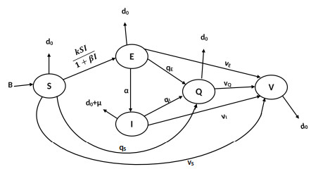
The susceptible, exposed, infected, quarantined and vaccinated (SEIQV) population is accounted for in a mathematical model of COVID-19. This model covers the therapy for diseased people as well as therapeutic measures like immunization for susceptible people to enable understanding of the dynamics of the disease's propagation. Each of the equilibrium points, i.e., disease-free and endemic, has been proven to be globally asymptotically stable under the assumption that $ \mathscr{R}_0 $ is smaller or larger than unity, respectively. Although vaccination coverage is high, the basic reproduction number depends on the vaccine's effectiveness in preventing disease when $ \mathscr{R}_0 > 0 $. The Jacobian matrix and the Routh-Hurwitz theorem are used to derive the aforementioned analysis techniques. The results are further examined numerically by using the standard second-order Runge-Kutta (RK2) method. In order to visualize the global dynamics of the aforementioned model, the proposed model is expanded to examine some piecewise fractional order derivatives. We may comprehend the crossover behavior in the suggested model's illness dynamics by using the relevant derivative. To numerical present the results, we use RK2 method.

| [1] | Naming the coronavirus disease (COVID-19) and the virus that causes it, Available from: World Health Organization (WHO), 2020, https://www.who.int/emergencies/diseases/novel-coronavirus-2019/technical-guidance/naming-the-coronavirus-disease-(covid-2019)-and-the-virus-that-causes-it. |
| [2] |
S. Zhao, S. S. Musa, Q. Lin, J. Ran, G. Yang, W. Wang, et al., Estimating the unreported number of novel coronavirus (2019-nCoV) cases in China in the first half of January 2020, a data-driven modelling analysis of the early outbreak, J. Clin. Med., 9 (2020), 388. https://doi.org/10.3390/jcm9020388 doi: 10.3390/jcm9020388

|
| [3] |
I. Nesteruk, Statistics based predictions of coronavirus 2019-nCoV spreading in mainland China, MedRxiv, 4 (2020), 1988–1989. https://doi.org/10.1101/2020.02.12.20021931 doi: 10.1101/2020.02.12.20021931
|
| [4] |
D. S. Hui, E. I. Azhar, T. A. Madani, F. Ntoumi, R. Kock, O. Dar, et al., The continuing 2019-nCoV epidemic threat of novel coronaviruses to global health–The latest 2019 novel coronavirus outbreak in Wuhan, China, Int. J. Infect. Dis., 91 (2020), 264–266. https://doi.org/10.1016/j.ijid.2020.01.009 doi: 10.1016/j.ijid.2020.01.009
|
| [5] |
S. Zhao, Q. Lin, J. Ran, S. S. Musa, G. Yang, W. Wang, et al., Preliminary estimation of the basic reproduction number of novel coronavirus (2019-nCoV) in China, Int. J. Infect. Dis., 92 (2020), 214–217. https://doi.org/10.1016/j.ijid.2020.01.050 doi: 10.1016/j.ijid.2020.01.050
|
| [6] |
K. Shah, R. Din, W. Deebani, P. Kumam, Z. Shah, On nonlinear classical and fractional order dynamical system addressing COVID-19, Results Phys., 24 (2021), 104069. https://doi.org/10.1016/j.rinp.2021.104069 doi: 10.1016/j.rinp.2021.104069
|
| [7] |
A. J. Lotka, Contribution to the theory of periodic reactions, J. Phys. Chem., 14 (1910), 271–274. https://doi.org/10.1021/j150111a004 doi: 10.1021/j150111a004
|
| [8] |
N. S. Goel, S. C. MAITRA, E. W. MONTROLL, On the Volterra and other nonlinear models of interacting populations, Rev. Mod. Phys., 43 (1971), 231. https://doi.org/10.1103/RevModPhys.43.231 doi: 10.1103/RevModPhys.43.231
|
| [9] |
P. Zhou, X. L. Yang, X. G. Wang, B. Hu, L. Zhang, W. Zhang, et al., A pneumonia outbreak associated with a new coronavirus of probable bat origin, Nature, 579 (2020), 270–273. https://doi.org/10.1038/s41586-020-2012-7 doi: 10.1038/s41586-020-2012-7
|
| [10] |
Q. Li, X. Guan, P. Wu, X. Wang, L. Zhou, Y. Tong, et al., Early transmission dynamics in Wuhan, China, of novel coronavirus infected pneumonia, N. Engl. J. Med., 382 (2020), 1199–1207. https://doi.org/10.1056/NEJMoa2001316 doi: 10.1056/NEJMoa2001316
|
| [11] |
I. I. Bogoch, A. Watts, A. Thomas-Bachli, C. Huber, M. U. G. Kraemer, K. Khan, Pneumonia of unknown aetiology in Wuhan, China: potential for international spread via commercial air travel, J. Travel Med., 27 (2020), taaa008. https://doi.org/10.1093/jtm/taaa008 doi: 10.1093/jtm/taaa008
|
| [12] |
C. Lu, H. Liu, D. Zhang, Dynamics and simulations of a second order stochastically perturbed SEIQV epidemic model with saturated incidence rate, Chaos Soliton. Fract., 152 (2021), 111312. https://doi.org/10.1016/j.chaos.2021.111312 doi: 10.1016/j.chaos.2021.111312
|
| [13] |
X. Liu, L. Yang, Stability analysis of a SEIQV epidemic model with saturated incidence rate, Nonlinear Anal. Real, 13 (2012), 2671–2679. https://doi.org/10.1016/j.nonrwa.2012.03.010 doi: 10.1016/j.nonrwa.2012.03.010
|
| [14] |
A. B. Gumel, S. Ruan, T. Day, J. Watmough, F. Brauer, P. van den Driessche, et al., Modelling strategies for controlling SARS out breaks, Proc. R. Soc. Lond. B, 271 (2004), 2223–2232. https://doi.org/10.1098/rspb.2004.2800 doi: 10.1098/rspb.2004.2800
|
| [15] |
A. Atangana, S. I. Araz, Modeling third waves of Covid-19 spread with piecewise differential and integral operators: Turkey, Spain and Czechia, Results Phys., 29 (2021), 104694. https://doi.org/10.1016/j.rinp.2021.104694 doi: 10.1016/j.rinp.2021.104694
|
| [16] |
Z. Zhang, A. Zeb, S. Hussain, E. Alzahrani, Dynamics of COVID-19 mathematical model with stochastic perturbation, Adv. Differ. Equ., 2020 (2020), 451. https://doi.org/10.1186/s13662-020-02909-1 doi: 10.1186/s13662-020-02909-1
|
| [17] |
A. Atangana, S. I. Araz, Mathematical model of COVID-19 spread in Turkey and South Africa: theory, methods, and applications, Adv. Differ. Equ., 2020 (2020), 659. https://doi.org/10.1186/s13662-020-03095-w doi: 10.1186/s13662-020-03095-w
|
| [18] |
N. H. Alharthi, M. B. Jeelani, A Fractional model of COVID-19 in the frame of environmental transformation with caputo fractional derivative, Adv. Appl. Stat., 88 (2023), 225–244. https://doi.org/10.17654/0972361723047 doi: 10.17654/0972361723047
|
| [19] |
M. B. Jeelani, Stability and computational analysis of COVID-19 using a higher order galerkin time discretization scheme, Adv. Appl. Stat., 86 (2023), 167–206. https://doi.org/10.17654/0972361723022 doi: 10.17654/0972361723022
|
| [20] |
C. A. B. Pearson, F. Bozzani, S. R. Procter, N. G. Davies, M. Huda, H. T. Jensen, et al., COVID-19 vaccination in Sindh Province, Pakistan: A modelling study of health impact and cost-effectiveness, PLoS Med., 18 (2021), e1003815. https://doi.org/10.1371/journal.pmed.1003815 doi: 10.1371/journal.pmed.1003815
|
| [21] |
R. P. Curiel, H. G. Ramírez, Vaccination strategies against COVID-19 and the diffusion of anti-vaccination views, Sci. Rep., 11 (2021), 6626. https://doi.org/10.1038/s41598-021-85555-1 doi: 10.1038/s41598-021-85555-1
|
| [22] |
J. T. Wu, K. Leung, G. M. Leung, Nowcasting and forecasting the potential domestic and international spread of the 2019-nCoV outbreak originating in Wuhan, China: a modelling study, The Lancet, 395 (2020), 689–697. https://doi.org/10.1016/S0140-6736(20)30260-9 doi: 10.1016/S0140-6736(20)30260-9
|
| [23] |
M. S. Arshad, D. Baleanu, M. B. Riaz, M. Abbas, A novel 2-stage fractional Runge-kutta method for a time-fractional logistic growth model, Discrete Dyn. Nat. Soc., 2000 (2000), 1020472. https://doi.org/10.1155/2020/1020472 doi: 10.1155/2020/1020472
|
| [24] |
T. Abdeljawad, Q. M. Al-Mdallal, F. Jarad, Fractional logistic models in the frame of fractional operators generated by conformable derivatives, Chaos Soliton. Fract., 119 (2019), 94–101. https://doi.org/10.1016/j.chaos.2018.12.015 doi: 10.1016/j.chaos.2018.12.015
|
| [25] |
O. A. Omar, R. A. Elbarkouky, H. M. Ahmed, Fractional stochastic modelling of COVID-19 under wide spread of vaccinations: Egyptian case study, Alex. Eng. J., 61 (2022), 8595–8609. https://doi.org/10.1016/j.aej.2022.02.002 doi: 10.1016/j.aej.2022.02.002
|
| [26] |
S. Saha, A. K. Saha, Modeling the dynamics of COVID-19 in the presence of Delta and Omicron variants with vaccination and non-pharmaceutical interventions, Heliyon, 9 (2023), e17900. https://doi.org/10.1016/j.heliyon.2023.e17900 doi: 10.1016/j.heliyon.2023.e17900
|
| [27] |
H. M. Ahmed, R. A. Elbarkouky, O. A. M. Omar, M. A. Ragusa, Models for COVID-19 daily confirmed cases in different countries, Mathematics, 9 (2021), 659. https://doi.org/10.3390/math9060659 doi: 10.3390/math9060659
|
| [28] |
F. Liu, K. Burrage, Novel techniques in parameter estimition for fractinal dynamical models arising from biological systems, Comput. Math. Appl., 62 (2011), 822–833. https://doi.org/10.1016/j.camwa.2011.03.002 doi: 10.1016/j.camwa.2011.03.002
|
| [29] | M. T. Hoang, O. F. Egbelowo, Dynamics of a fractional-order hepatitis b epidemic model and its solutions by nonstandard numerical schemes, In: Mathematical modelling and analysis of infectious diseases, Cham: Springer, 2020,127–153. https://doi.org/10.1007/978-3-030-49896-2_5 |
| [30] |
A. Zeb, E. Alzahrani, V. S. Erturk, G. Zaman, Mathematical model for coronavirus disease 2019 (COVID-19) containing isolation class, BioMed Res. Int., 2020 (2020), 3452402. https://doi.org/10.1155/2020/3452402 doi: 10.1155/2020/3452402
|
| [31] |
K. Shah, A. Ali, S. Zeb, A. Khan, M. A. Alqudah, T. Abdeljawad, Study of fractional order dynamics of nonlinear mathematical model, Alex. Eng. J., 61 (2022), 11211–11224. https://doi.org/10.1016/j.aej.2022.04.039 doi: 10.1016/j.aej.2022.04.039
|
| [32] |
S. Boccaletti, W. Ditto, G. Mindlin, A. Atangana, Modeling and forecasting of epidemic spreading: The case of Covid-19 and beyond, Chaos Soliton. Fract., 135 (2020), 109794. https://doi.org/10.1016/j.chaos.2020.109794 doi: 10.1016/j.chaos.2020.109794
|
| [33] |
E. Atangana, A. Atangana, Facemasks simple but powerful weapons to protect against COVID-19 spread: Can they have sides effects, Results Phys., 19 (2020), 103425. https://doi.org/10.1016/j.rinp.2020.103425 doi: 10.1016/j.rinp.2020.103425
|
| [34] |
S. T. M. Thabet, M. S. Abdo, K. Shah, T. Abdeljawad, Study of transmission dynamics of COVID-19 mathematical model under ABC fractional order derivative, Results Phys., 19 (2020), 103507. https://doi.org/10.1016/j.rinp.2020.103507 doi: 10.1016/j.rinp.2020.103507
|
| [35] |
A. Al Elaiw, F. Hafeez, M. B. Jeelani, M. Awadalla, K. Abuasbeh, Existence and uniqueness results for mixed derivative involving fractional operators, AIMS Mathematics, 8 (2023), 7377–7393. https://doi.org/10.3934/math.2023371 doi: 10.3934/math.2023371
|
| [36] |
A. Moumen, R. Shafqat, A. Alsinai, H. Boulares, M. Cancan, M. B. Jeelani, Analysis of fractional stochastic evolution equations by using Hilfer derivative of finite approximate controllability, AIMS Mathematics, 8 (2023), 16094–16114. https://doi.org/10.3934/math.2023821 doi: 10.3934/math.2023821
|
| [37] |
J. T. Machado, V. Kiryakova, F. Mainardi, Recent history of fractional calculus, Commun. Nonlinear Sci., 16 (2011), 1140–1153. https://doi.org/10.1016/j.cnsns.2010.05.027 doi: 10.1016/j.cnsns.2010.05.027
|
| [38] |
F. C. Meral, T. J. Royston, R. Magin, Fractional calculus in viscoelasticity: an experimental study, Commun. Nonlinear Sci., 15 (2010), 939–945. https://doi.org/10.1016/j.cnsns.2009.05.004 doi: 10.1016/j.cnsns.2009.05.004
|
| [39] |
L. M. Richard, Fractional calculus in bioengineering, part 1, Critical Reviews in Biomedical Engineering, 32 (2004), 104. https://doi.org/10.1615/CritRevBiomedEng.v32.i1.10 doi: 10.1615/CritRevBiomedEng.v32.i1.10
|
| [40] | M. Dalir, M. Bashour, Applications of fractional calculus, Appl. Math. Sci., 4 (2010), 1021–1032. |
| [41] |
A. S. Alnahdi, M. B. Jeelani, H. A. Wahash, M. A. Abdulwasaa, A Detailed Mathematical Analysis of the Vaccination Model for COVID-19, Computer Modeling in Engineering Sciences, 135 (2022), 1315–1343. https://doi.org/10.32604/cmes.2022.023694 doi: 10.32604/cmes.2022.023694
|
| [42] | K. Dehingia, M. B. Jeelani, A. Das, Artificial intelligence and machine learning: A smart science approach for cancer control, In: Advances in deep learning for medical image analysis, Boca Raton: CRC Press, 2022. https://doi.org/10.1201/9781003230540 |
| [43] |
M. B. Jeelani, A. S. Alnahdi, M. A. Almalahi, M. S. Abdo, H. A. Wahash, N. H. Alharthi, Qualitative analyses of fractional integro-differential equations with a variable order under the Mittag-Leffler power law, J. Funct. Space., 2022 (2022), 6387351. https://doi.org/10.1155/2022/6387351 doi: 10.1155/2022/6387351
|
| [44] | R. L. Magin, Fractional calculus in bioengineering: A tool to model complex dynamics, In: Proceedings of the 13th International Carpathian Control Conference (ICCC), High Tatras, Slovakia, 2012,464–469. https://doi.org/10.1109/CarpathianCC.2012.6228688 |
| [45] | Y. A. Rossikhin, M. V. Shitikova, Applications of fractional calculus to dynamic problems of linear and nonlinear hereditary mechanics of solids, 50 (1997), 15–67. https://doi.org/10.1115/1.3101682 |
| [46] | A. Carpinteri, F. Mainardi, Fractals and fractional calculus in continuum mechanics, Vienna: Springer, 1997. https://doi.org/10.1007/978-3-7091-2664-6 |
| [47] |
L. M. Richard, Fractional calculus models of complex dynamics in biological tissues, Comput. Math. Appl., 59 (2010), 1586–1593. https://doi.org/10.1016/j.camwa.2009.08.039 doi: 10.1016/j.camwa.2009.08.039
|
| [48] |
M. Shimizu, W. Zhang, Fractional calculus approach to dynamic problems of viscoelastic materials, JSME International Journal Series C Mechanical Systems, Machine Elements and Manufacturing, 42 (1999), 825–837. https://doi.org/10.1299/jsmec.42.825 doi: 10.1299/jsmec.42.825
|
| [49] |
F. Mainardi, An historical perspective on fractional calculus in linear viscoelasticity, Fract. Calc. Appl. Anal., 15 (2012), 712–717. https://doi.org/10.2478/s13540-012-0048-6 doi: 10.2478/s13540-012-0048-6
|
| [50] |
Z. Dai, Y. Peng, H. A. Mansy, R. H. Sandler, T. J. Royston, A model of lung parenchyma stress relaxation using fractional viscoelasticity, Med. Eng. Phys., 37 (2015), 752–758. https://doi.org/10.1016/j.medengphy.2015.05.003 doi: 10.1016/j.medengphy.2015.05.003
|
| [51] |
M. A. Matlob, Y. Jamali, The concepts and applications of fractional order differential calculus in modeling of viscoelastic systems, Critical Reviews in Biomedical Engineering, 47 (2019), 249–276. https://doi.org/10.1615/CritRevBiomedEng.2018028368 doi: 10.1615/CritRevBiomedEng.2018028368
|
| [52] |
W. Grzesikiewicz, A. Wakulicz, A. Zbiciak, Non-linear problems of fractional calculus in modeling of mechanical systems, Int. J. Mech. Sci., 70 (2013), 90–98. https://doi.org/10.1016/j.ijmecsci.2013.02.007 doi: 10.1016/j.ijmecsci.2013.02.007
|
| [53] |
C. Celauro, C. Fecarotti, A. Pirrotta, A. C. Collop, Experimental validation of a fractional model for creep/recovery testing of asphalt mixtures, Constr. Build. Mater., 36 (2012), 458–466. https://doi.org/10.1016/j.conbuildmat.2012.04.028 doi: 10.1016/j.conbuildmat.2012.04.028
|
| [54] |
W. Adel, A. Elsonbaty, A. Aldurayhim, A. El-Mesady, Investigating the dynamics of a novel fractional-order monkeypox epidemic model with optimal control, Alex. Eng. J., 73 (2023), 519–542. https://doi.org/10.1016/j.aej.2023.04.051 doi: 10.1016/j.aej.2023.04.051
|
| [55] |
A. El-Mesady, A. Elsonbaty, W. Adel, On nonlinear dynamics of a fractional order monkeypox virus model, Chaos Soliton. Fract., 164 (2022), 112716. https://doi.org/10.1016/j.chaos.2022.112716 doi: 10.1016/j.chaos.2022.112716
|
| [56] |
N. Ahmed, A. Elsonbaty, A. Raza, M. Rafiq, W. Adel, Numerical simulation and stability analysis of a novel reaction-diffusion COVID-19 model, Nonlinear Dyn., 106 (2021), 1293–1310. https://doi.org/10.1007/s11071-021-06623-9 doi: 10.1007/s11071-021-06623-9
|
| [57] |
A. M. R. Elsonbaty, Z. Sabir, R. Ramaswamy, W. Adel, Dynamical analysis of a novel discrete fractional SITRS model for COVID-19, Fractals, 29 (2021), 2140035. https://doi.org/10.1142/S0218348X21400351 doi: 10.1142/S0218348X21400351
|
| [58] |
A. El-Mesady, A. Waleed Adel, A. A. Elsadany, A. Elsonbaty, Stability analysis and optimal control strategies of a fractional-order Monkeypox virus infection model, Phys. Scr., 98 (2023), 095256. https://doi.org/10.1088/1402-4896/acf16f doi: 10.1088/1402-4896/acf16f
|
| [59] |
M. M. Khalsaraei, An improvement on the positivity results for 2-stage explicit Runge-Kutta methods, J. Comput. Appl. Math., 235 (2010), 137–143. https://doi.org/10.1016/j.cam.2010.05.020 doi: 10.1016/j.cam.2010.05.020
|
| [60] |
Z. J. Fu, Z. C. Tang, H. T. Zhao, P. W. Li, T. Rabczuk, Numerical solutions of the coupled unsteady nonlinear convection-diffusion equations based on generalized finite difference method, Eur. Phys. J. Plus, 134 (2019), 272. https://doi.org/10.1140/epjp/i2019-12786-7 doi: 10.1140/epjp/i2019-12786-7
|
| [61] |
A. Atangana, S. I. Araz, New concept in calculus: piecewise differential and integral operators, Chaos Soliton. Fract., 145 (2021), 110638. https://doi.org/10.1016/j.chaos.2020.110638 doi: 10.1016/j.chaos.2020.110638
|
| [62] | Current information about COVID-19 in Pakistan, 2021, Available from: https://www.worldometers.info. |
| [63] | Pakistan COVID-19 Corona tracker, 2021, Available from: https://www.coronatracker.com/country/pakistan/. |
| [64] |
F. Chamchod, N. F. Britton, On the dynamics of a two-strain influenza model with isolation, Math. Model. Nat. Phenom., 7 (2012), 49–61. https://doi.org/10.1051/mmnp/20127305 doi: 10.1051/mmnp/20127305
|
| [65] | Pakistan population, Available from: Worldometer, https://www.worldometers.info/world-population/pakistan-population/. |
| [66] |
S. Ahmad, A. Ullah, Q. M. Al-Mdallal, H. Khan, K. Shah, A. Khan, Fractional order mathematical modeling of COVID-19 transmission, Chaos Soliton. Fract., 139 (2020), 110256. https://doi.org/10.1016/j.chaos.2020.110256 doi: 10.1016/j.chaos.2020.110256
|
| [67] | Vaccines, Available from: UNICEF Pakistan, https://www.unicef.org/pakistan/topics/vaccines |
| [68] |
S. Mwalili, M. Kimathi, V. Ojiambo, D. Gathungu, R. Mbogo, SEIR model for COVID-19 dynamics incorporating the environment and social distancing, BMC Res. Notes, 13 (2020), 352. https://doi.org/10.1186/s13104-020-05192-1 doi: 10.1186/s13104-020-05192-1
|


Figures(18) / Tables(2)

Mdi Begum Jeelani, Abeer S Alnahdi, Rahim Ud Din, Hussam Alrabaiah, Azeem Sultana. Mathematical model to investigate transmission dynamics of COVID-19 with vaccinated class[J]. AIMS Mathematics, 2023, 8(12): 29932-29955. doi: 10.3934/math.20231531


 DownLoad: