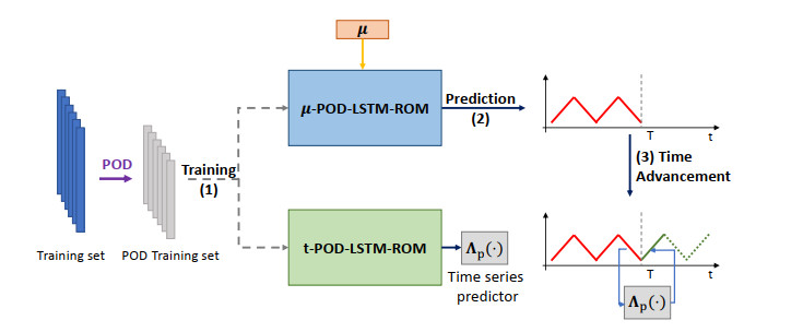
Deep learning-based reduced order models (DL-ROMs) have been recently proposed to overcome common limitations shared by conventional ROMs–built, e.g., through proper orthogonal decomposition (POD)–when applied to nonlinear time-dependent parametrized PDEs. In particular, POD-DL-ROMs can achieve an extremely good efficiency in the training stage and faster than real-time performances at testing, thanks to a prior dimensionality reduction through POD and a DL-based prediction framework. Nonetheless, they share with conventional ROMs unsatisfactory performances regarding time extrapolation tasks. This work aims at taking a further step towards the use of DL algorithms for the efficient approximation of parametrized PDEs by introducing the $ \mu t $-POD-LSTM-ROM framework. This latter extends the POD-DL-ROMs by adding a two-fold architecture taking advantage of long short-term memory (LSTM) cells, ultimately allowing long-term prediction of complex systems' evolution, with respect to the training window, for unseen input parameter values. Numerical results show that $ \mu t $-POD-LSTM-ROMs enable the extrapolation for time windows up to 15 times larger than the training time interval, also achieving better performances at testing than POD-DL-ROMs.
Citation: Stefania Fresca, Federico Fatone, Andrea Manzoni. Long-time prediction of nonlinear parametrized dynamical systems by deep learning-based reduced order models[J]. Mathematics in Engineering, 2023, 5(6): 1-36. doi: 10.3934/mine.2023096
Deep learning-based reduced order models (DL-ROMs) have been recently proposed to overcome common limitations shared by conventional ROMs–built, e.g., through proper orthogonal decomposition (POD)–when applied to nonlinear time-dependent parametrized PDEs. In particular, POD-DL-ROMs can achieve an extremely good efficiency in the training stage and faster than real-time performances at testing, thanks to a prior dimensionality reduction through POD and a DL-based prediction framework. Nonetheless, they share with conventional ROMs unsatisfactory performances regarding time extrapolation tasks. This work aims at taking a further step towards the use of DL algorithms for the efficient approximation of parametrized PDEs by introducing the $ \mu t $-POD-LSTM-ROM framework. This latter extends the POD-DL-ROMs by adding a two-fold architecture taking advantage of long short-term memory (LSTM) cells, ultimately allowing long-term prediction of complex systems' evolution, with respect to the training window, for unseen input parameter values. Numerical results show that $ \mu t $-POD-LSTM-ROMs enable the extrapolation for time windows up to 15 times larger than the training time interval, also achieving better performances at testing than POD-DL-ROMs.

| [1] |
P. Benner, S. Gugercin, K. Willcox, A survey of projection-based model reduction methods for parametric dynamical systems, SIAM Rev., 57 (2015), 483–531. https://doi.org/10.1137/130932715 doi: 10.1137/130932715

|
| [2] | A. Quarteroni, A. Manzoni, F. Negri, Reduced basis methods for partial differential equations: an introduction, Springer, 2016. https://doi.org/10.1007/978-3-319-15431-2 |
| [3] | P. Benner, A. Cohen, M. Ohlberger, K. Willcox, Model reduction and approximation: theory and algorithms, SIAM, 2017. |
| [4] | A. Quarteroni, A. Valli, Numerical approximation of partial differential equations, Springer, 1994. https://doi.org/10.1007/978-3-540-85268-1 |
| [5] |
A. Manzoni, An efficient computational framework for reduced basis approximation and a posteriori error estimation of parametrized Navier-Stokes flows, ESAIM: Math. Modell. Numer. Anal., 48 (2014), 1199–1226. https://doi.org/10.1051/m2an/2014013 doi: 10.1051/m2an/2014013
|
| [6] |
F. Ballarin, A. Manzoni, A. Quarteroni, G. Rozza, Supremizer stabilization of POD-Galerkin approximation of parametrized steady incompressible Navier-Stokes equations, Int. J. Numer. Meth. Eng., 102 (2015), 1136–1161. https://doi.org/10.1002/nme.4772 doi: 10.1002/nme.4772
|
| [7] |
N. Dal Santo, A. Manzoni, Hyper-reduced order models for parametrized unsteady Navier-Stokes equations on domains with variable shape, Adv. Comput. Math., 45 (2019), 2463–2501. https://doi.org/10.1007/s10444-019-09722-9 doi: 10.1007/s10444-019-09722-9
|
| [8] | C. Farhat, S. Grimberg, A. Manzoni, A. Quarteroni, Computational bottlenecks for PROMs: pre-computation and hyperreduction, In: P. Benner, S. Grivet-Talocia, A. Quarteroni, G. Rozza, W. Schilders, L. Silveira, Model order reduction: volume 2: snapshot-based methods and algorithms, Boston: De Gruyter, 2020,181–244. https://doi.org/10.1515/9783110671490-005 |
| [9] |
G. Gobat, A. Opreni, S. Fresca, A. Manzoni, A. Frangi, Reduced order modeling of nonlinear microstructures through proper orthogonal decomposition, Mech. Syst. Signal Process., 171 (2022), 108864. https://doi.org/10.1016/j.ymssp.2022.108864 doi: 10.1016/j.ymssp.2022.108864
|
| [10] |
I. Lagaris, A. Likas, D. Fotiadis, Artificial neural networks for solving ordinary and partial differential equations, IEEE Trans. Neur. Net., 9 (1998), 987–1000. https://doi.org/10.1109/72.712178 doi: 10.1109/72.712178
|
| [11] |
L. Aarts, P. van der Veer, Neural network method for solving partial differential equations, Neural Process. Lett., 14 (2001), 261–271. https://doi.org/10.1023/A:1012784129883 doi: 10.1023/A:1012784129883
|
| [12] |
K. Hornik, Approximation capabilities of multilayer feedforward networks, Neural Networks, 4 (1991), 251–257. https://doi.org/10.1016/0893-6080(91)90009-T doi: 10.1016/0893-6080(91)90009-T
|
| [13] |
Y. Khoo, J. Lu, L. Ying, Solving parametric PDE problems with artificial neural networks, Eur. J. Appl. Math., 32 (2021), 421–435. https://doi.org/10.1017/S0956792520000182 doi: 10.1017/S0956792520000182
|
| [14] |
C. Michoski, M. Milosavljević, T. Oliver, D. Hatch, Solving differential equations using deep neural networks, Neurocomputing, 399 (2020), 193–212. https://doi.org/10.1016/j.neucom.2020.02.015 doi: 10.1016/j.neucom.2020.02.015
|
| [15] |
J. Berg, K. Nyström, Data-driven discovery of PDEs in complex datasets, J. Comput. Phys., 384 (2019), 239–252. https://doi.org/10.1016/j.jcp.2019.01.036 doi: 10.1016/j.jcp.2019.01.036
|
| [16] |
M. Raissi, P. Perdikaris, G. Karniadakis, Physics-informed neural networks: a deep learning framework for solving forward and inverse problems involving nonlinear partial differential equations, J. Comput. Phys., 378 (2019), 686–707. https://doi.org/10.1016/j.jcp.2018.10.045 doi: 10.1016/j.jcp.2018.10.045
|
| [17] |
M. Raissi, Deep hidden physics models: deep learning of nonlinear partial differential equations, J. Mach. Learn. Res., 19 (2018), 932–955. https://doi.org/10.5555/3291125.3291150 doi: 10.5555/3291125.3291150
|
| [18] |
J. A. A. Opschoor, P. C. Petersen, C. Schwab, Deep ReLU networks and high-order finite element methods, Anal. Appl., 18 (2020), 715–770. https://doi.org/10.1142/S0219530519410136 doi: 10.1142/S0219530519410136
|
| [19] |
G. Kutyniok, P. Petersen, M. Raslan, R. Schneider, A theoretical analysis of deep neural networks and parametric PDEs, Constr. Approx., 55 (2021), 73–125. https://doi.org/10.1007/s00365-021-09551-4 doi: 10.1007/s00365-021-09551-4
|
| [20] |
D. Yarotsky, Error bounds for approximations with deep relu networks, Neural Networks, 94 (2017), 103–114. https://doi.org/10.1016/j.neunet.2017.07.002 doi: 10.1016/j.neunet.2017.07.002
|
| [21] |
N. Franco, A. Manzoni, P. Zunino, A deep learning approach to reduced order modelling of parameter dependent partial differential equations, Math. Comp., 92 (2023), 483–524. https://doi.org/10.1090/mcom/3781 doi: 10.1090/mcom/3781
|
| [22] | T. De Ryck, S. Mishra, Generic bounds on the approximation error for physics-informed (and) operator learning, arXiv, 2022. https://doi.org/10.48550/arXiv.2205.11393 |
| [23] |
N. Kovachki, S. Lanthaler, S. Mishra, On universal approximation and error bounds for Fourier neural operators, J. Mach. Learn. Res., 22 (2021), 13237–13312. https://doi.org/10.5555/3546258.3546548 doi: 10.5555/3546258.3546548
|
| [24] |
S. Lanthaler, S. Mishra, G. E. Karniadakis, Error estimates for DeepONets: a deep learning framework in infinite dimensions, Trans. Math. Appl., 6 (2022), tnac001. https://doi.org/10.1093/imatrm/tnac001 doi: 10.1093/imatrm/tnac001
|
| [25] |
M. Guo, J. S. Hesthaven, Reduced order modeling for nonlinear structural analysis using gaussian process regression, Comput. Methods Appl. Mech. Eng., 341 (2018), 807–826. https://doi.org/10.1016/j.cma.2018.07.017 doi: 10.1016/j.cma.2018.07.017
|
| [26] |
M. Guo, J. S. Hesthaven, Data-driven reduced order modeling for time-dependent problems, Comput. Methods Appl. Mech. Eng., 345 (2019), 75–99. https://doi.org/10.1016/j.cma.2018.10.029 doi: 10.1016/j.cma.2018.10.029
|
| [27] |
J. S. Hesthaven, S. Ubbiali, Non-intrusive reduced order modeling of nonlinear problems using neural networks, J. Comput. Phys., 363 (2018), 55–78. https://doi.org/10.1016/j.jcp.2018.02.037 doi: 10.1016/j.jcp.2018.02.037
|
| [28] |
S. Pawar, S. E. Ahmed, O. San, A. Rasheed, Data-driven recovery of hidden physics in reduced order modeling of fluid flows, Phys. Fluids, 32 (2020), 036602. https://doi.org/10.1063/5.0002051 doi: 10.1063/5.0002051
|
| [29] |
B. A. Freno, K. T. Carlberg, Machine-learning error models for approximate solutions to parameterized systems of nonlinear equations, Comput. Methods Appl. Mech. Eng., 348 (2019) 250–296. https://doi.org/10.1016/j.cma.2019.01.024 doi: 10.1016/j.cma.2019.01.024
|
| [30] | E. J. Parish, K. T. Carlberg, Time-series machine learning error models for appproximate solutions to dynamical systems, $15^{th}$ National Congress of Computational Mechanics, 2019. |
| [31] |
K. Lee, K. T. Carlberg, Model reduction of dynamical systems on nonlinear manifolds using deep convolutional autoencoders, J. Comput. Phys., 404 (2020), 108973. https://doi.org/10.1016/j.jcp.2019.108973 doi: 10.1016/j.jcp.2019.108973
|
| [32] |
S. Fresca, L. Dedè, A. Manzoni, A comprehensive deep learning-based approach to reduced order modeling of nonlinear time-dependent parametrized PDEs, J. Sci. Comput., 87 (2021), 61. https://doi.org/10.1007/s10915-021-01462-7 doi: 10.1007/s10915-021-01462-7
|
| [33] |
S. Fresca, A. Manzoni, POD-DL-ROM: enhancing deep learning-based reduced order models for nonlinear parametrized PDEs by proper orthogonal decomposition, Comput. Methods Appl. Mech. Eng., 388 (2021), 114181. https://doi.org/10.1016/j.cma.2021.114181 doi: 10.1016/j.cma.2021.114181
|
| [34] |
N. Halko, P. G. Martinsson, J. A. Tropp, Finding structure with randomness: probabilistic algorithms for constructing approximate matrix decompositions, SIAM Rev., 53 (2011), 217–288. https://doi.org/10.1137/090771806 doi: 10.1137/090771806
|
| [35] |
S. Fresca, A. Manzoni, L. Dedè, A. Quarteroni, Deep learning-based reduced order models in cardiac electrophysiology, PLoS One, 15 (2020), e0239416. https://doi.org/10.1371/journal.pone.0239416 doi: 10.1371/journal.pone.0239416
|
| [36] |
S. Fresca, A. Manzoni, L. Dedè, A. Quarteroni, POD-enhanced deep learning-based reduced order models for the real-time simulation of cardiac electrophysiology in the left atrium, Front. Physiol., 12 (2021), 679076. https://doi.org/10.3389/fphys.2021.679076 doi: 10.3389/fphys.2021.679076
|
| [37] |
S. Fresca, A. Manzoni, Real-time simulation of parameter-dependent fluid flows through deep learning-based reduced order models, Fluids, 6 (2021), 259. https://doi.org/10.3390/fluids6070259 doi: 10.3390/fluids6070259
|
| [38] |
S. Fresca, G. Gobat, P. Fedeli, A. Frangi, A. Manzoni, Deep learning-based reduced order models for the real-time simulation of the nonlinear dynamics of microstructures, Int. J. Numer. Methods Eng., 123 (2022), 4749–4777. https://doi.org/10.1002/nme.7054 doi: 10.1002/nme.7054
|
| [39] |
S. Hochreiter, J. Schmidhuber, Long short-term memory, Neural Comput., 9 (1997), 1735–1780. https://doi.org/10.1162/neco.1997.9.8.1735 doi: 10.1162/neco.1997.9.8.1735
|
| [40] |
F. Gers, J. Schmidhuber, F. Cummins, Learning to forget: continual prediction with LSTM, Neural Comput., 12 (2000), 2451–71. https://doi.org/10.1162/089976600300015015 doi: 10.1162/089976600300015015
|
| [41] | P. Sentz, K. Beckwith, E. C. Cyr, L. N. Olson, R. Patel, Reduced basis approximations of parameterized dynamical partial differential equations via neural networks, arXiv, 2021. https://doi.org/10.48550/arXiv.2110.10775 |
| [42] |
R. Maulik, B. Lusch, P. Balaprakash, Reduced-order modeling of advection-dominated systems with recurrent neural networks and convolutional autoencoders, Phys. Fluids, 33 (2021), 037106. https://doi.org/10.1063/5.0039986 doi: 10.1063/5.0039986
|
| [43] |
J. Xu, K. Duraisamy, Multi-level convolutional autoencoder networks for parametric prediction of spatio-temporal dynamics, Comput. Methods Appl. Mech. Eng., 372 (2020), 113379. https://doi.org/10.1016/j.cma.2020.113379 doi: 10.1016/j.cma.2020.113379
|
| [44] |
N. T. Mücke, S. M. Bohté, C. W. Oosterlee, Reduced order modeling for parameterized time-dependent pdes using spatially and memory aware deep learning, J. Comput. Sci., 53 (2021), 101408. https://doi.org/10.1016/j.jocs.2021.101408 doi: 10.1016/j.jocs.2021.101408
|
| [45] |
Y. Hua, Z. Zhao, R. Li, X. Chen, Z. Liu, H. Zhang, Deep learning with long short-term memory for time series prediction, IEEE Commun. Mag., 57 (2019), 114–119. https://doi.org/10.1109/MCOM.2019.1800155 doi: 10.1109/MCOM.2019.1800155
|
| [46] |
R. Maulik, B. Lusch, P. Balaprakash, Non-autoregressive time-series methods for stable parametric reduced-order models, Phys. Fluids, 32 (2020), 087115. https://doi.org/10.1063/5.0019884 doi: 10.1063/5.0019884
|
| [47] | N. Srivastava, E. Mansimov, R. Salakhutdinov, Unsupervised learning of video representations using LSTMs, ICML'15: Proceedings of the 32nd International Conference on International Conference on Machine Learning, 37 (2015), 843–852. |
| [48] |
P. Drineas, R. Kannan, M. W. Mahoney, Fast Monte Carlo algorithms for matrices Ⅱ: computing a low-rank approximation to a matrix, SIAM J. Comput., 36 (2006), 158–183. https://doi.org/10.1137/S0097539704442696 doi: 10.1137/S0097539704442696
|
| [49] |
M. Sangiorgio, F. Dercole, Robustness of LSTM neural networks for multi-step forecasting of chaotic time series, Chaos Soliton. Fract., 39 (2020), 110045. https://doi.org/10.1016/j.chaos.2020.110045 doi: 10.1016/j.chaos.2020.110045
|
| [50] | S. Du, T. Li, S. Horng, Time series forecasting using sequence-to-sequence deep learning framework, 2018 9th International Symposium on Parallel Architectures, Algorithms and Programming (PAAP), 2018,171–176. https://doi.org/10.1109/PAAP.2018.00037 |
| [51] | W. Zucchini, I. Macdonald, Hidden Markov models for time series: an introduction using R, 1 Ed., New York: Chapman and Hall/CRC, 2009. https://doi.org/10.1201/9781420010893 |
| [52] | P. Dostál, Forecasting of time series with fuzzy logic, In: I. Zelinka, G. Chen, O. E. Rössler, V. Snasel, A. Abraham, Nostradamus 2013: prediction, modeling and analysis of complex systems, Heidelberg: Springer, 210 (2013), 155–161. https://doi.org/10.1007/978-3-319-00542-3_16 |
| [53] | F. A. Gers, D. Eck, J. Schmidhuber, Applying LSTM to time series predictable through time-window approaches, In: G. Dorffner, H. Bischof, K. Hornik, Artificial neural networks — ICANN 2001, Lecture Notes in Computer Science, Springer, 2130 (2001), 669–676. https://doi.org/10.1007/3-540-44668-0_93 |
| [54] | S. Siami-Namini, N. Tavakoli, A. Siami Namin, A comparison of ARIMA and LSTM in forecasting time series, 2018 17th IEEE International Conference on Machine Learning and Applications (ICMLA), 2018, 1394–1401. https://doi.org/10.1109/ICMLA.2018.00227 |
| [55] | R. T. Q. Chen, Y. Rubanova, J. Bettencourt, D. Duvenaud, Neural ordinary differential equations, NIPS'18: Proceedings of the 32nd International Conference on Neural Information Processing Systems, 2018, 6572–6583. https://doi.org/10.5555/3327757.3327764 |
| [56] | S. Massaroli, M. Poli, J. Park, A. Yamashita, H. Asama, Dissecting neural ODEs, arXiv, 2021. https://doi.org/10.48550/arXiv.2002.08071 |
| [57] |
P. R. Vlachas, W. Byeon, Z. Y. Wan, T. P. Sapsis, P. Koumoutsakos, Data-driven forecasting of high-dimensional chaotic systems with long short-term memory networks, Proc. R. Soc. A: Math. Phys. Eng. Sci., 474 (2018), 1–20. https://doi.org/10.1098/rspa.2017.0844 doi: 10.1098/rspa.2017.0844
|
| [58] | D. P. Kingma, J. Ba, ADAM: a method for stochastic optimization, 3rd International Conference for Learning Representations, San Diego, 2015. |
| [59] | I. Goodfellow, Y. Bengio, A. Courville, Deep learning, MIT Press, 2016. Available from: http://www.deeplearningbook.org. |
| [60] | D. Clevert, T. Unterthiner, S. Hochreiter, Fast and accurate deep network learning by exponential linear units (ELUs), arXiv, 2015. https://doi.org/10.48550/arXiv.1511.07289 |
| [61] | K. He, X. Zhang, S. Ren, J. Sun, Delving deep into rectifiers: Surpassing human-level performance on ImageNet classification, Proceedings of the IEEE International Conference on Computer Vision (ICCV), 2015, 1026–1034. |
| [62] | M. Abadi, A. Agarwal, P. Barham, E. Brevdo, Z. Chen, C. Citro, et al., TensorFlow: large-scale machine learning on heterogeneous systems, 2015. Available from: https://www.tensorflow.org. |
| [63] | F. Negri, redbkit v2.2, 2017. Available from: https://github.com/redbKIT/redbKIT. |
| [64] |
J. Bergstra, Y. Bengio, Random search for hyper-parameter optimization, J. Mach. Learn. Res., 13 (2012), 281–305. https://doi.org/10.5555/2188385.2188395 doi: 10.5555/2188385.2188395
|
| [65] |
S. Chaturantabut, D. C. Sorensen, Discrete empirical interpolation for nonlinear model reduction, Proceedings of the 48h IEEE Conference on Decision and Control (CDC) held jointly with 2009 28th Chinese Control Conference, 2009, 4316–4321. https://doi.org/10.1109/CDC.2009.5400045 doi: 10.1109/CDC.2009.5400045
|
| [66] | C. M. Bishop, Neural networks for pattern recognition, Oxford University Press, Inc., 1995. |


Figures(12) / Tables(7)

Stefania Fresca, Federico Fatone, Andrea Manzoni. Long-time prediction of nonlinear parametrized dynamical systems by deep learning-based reduced order models[J]. Mathematics in Engineering, 2023, 5(6): 1-36. doi: 10.3934/mine.2023096


 DownLoad: