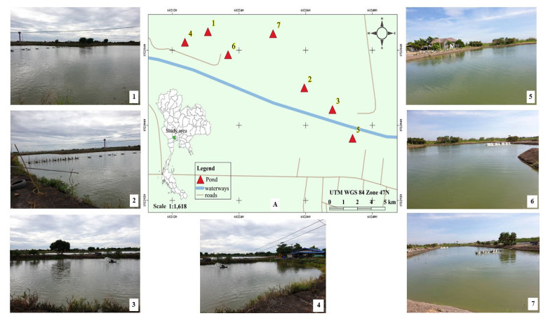
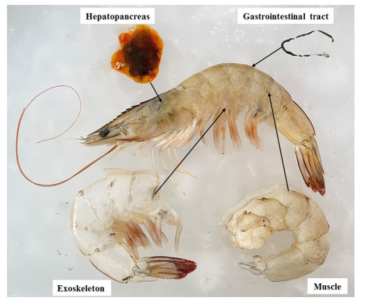
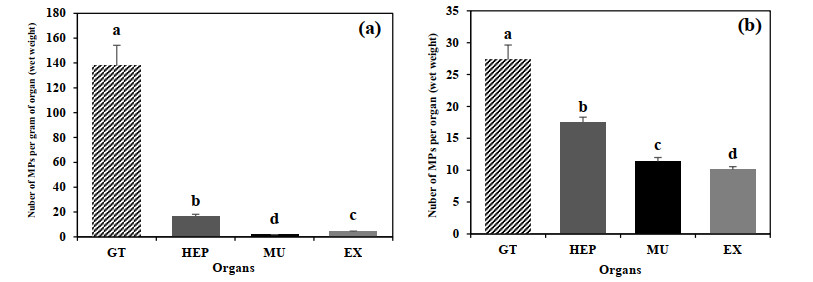
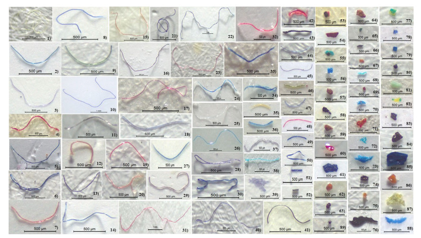
The presence of microplastics in commercially important seafood species is a new issue of food safety concern. Although plastic debris has been found in the gastrointestinal tracts of several species, the prevalence of microplastics in edible shrimp tissues in Thailand has not yet been established. For the first time, the gastrointestinal tract (GT), heptapancreas (HEP), muscle (MU) and exoskeleton (EX) of farmed white leg shrimp (Litopenaeus vannamei) from commercial aquaculture facilities in Nakhon Pathom Province, Thailand, were analyzed for microplastics (MPs). The number of MP items per tissue was 27.36±2.28 in the GT, 17.42±0.90 in the HEP, 11.37±0.60 in the MU and 10.04±0.52 in the EX. MP concentrations were 137.78±16.48, 16.31±1.87, 1.69±0.13 and 4.37±0.27 items/gram (ww) in the GT, HEP, MU and EX, respectively. Microplastics ranged in size from < 100 to 200–250 μm, with fragment-shape (62.07%), fibers (37.31%) and blue (43.69%) was the most common. The most frequently found polymers in shrimp tissue organs and pond water were polyethylene terephthalate (PET), polyvinyl acetate (PVAc) and cellulose acetate butyrate (CAB). Shrimp consumption (excluding GT and EX) was calculated as 28.79 items/shrimp/person/day using Thailand's consumption of shrimp, MP abundance and shrimp consumption. The results of the study can be used as background data for future biomonitoring of microplastics in shrimp species that are significant from an ecological and commercial perspective. MP abundance in farmed L. vannamei may be related to feeding habits and the source of MPs could come from the aquaculture facilities operations.
Citation: Akekawat Vitheepradit, Taeng-On Prommi. Microplastics in surface water and tissue of white leg shrimp, Litopenaeus vannamei, in a cultured pond in Nakhon Pathom Province, Central Thailand[J]. AIMS Environmental Science, 2023, 10(4): 478-503. doi: 10.3934/environsci.2023027
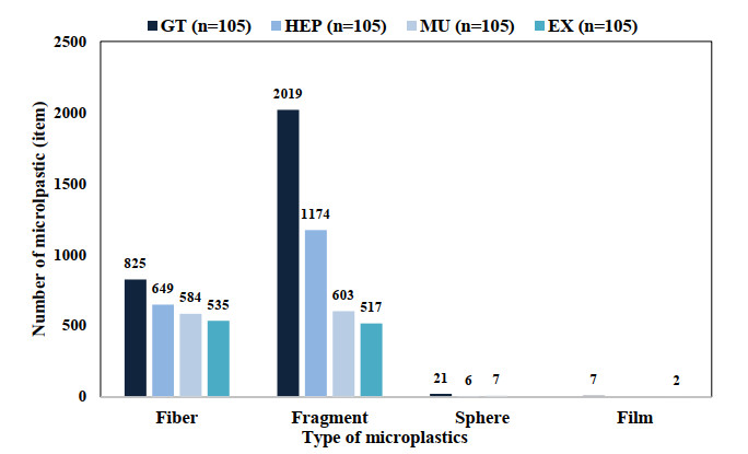
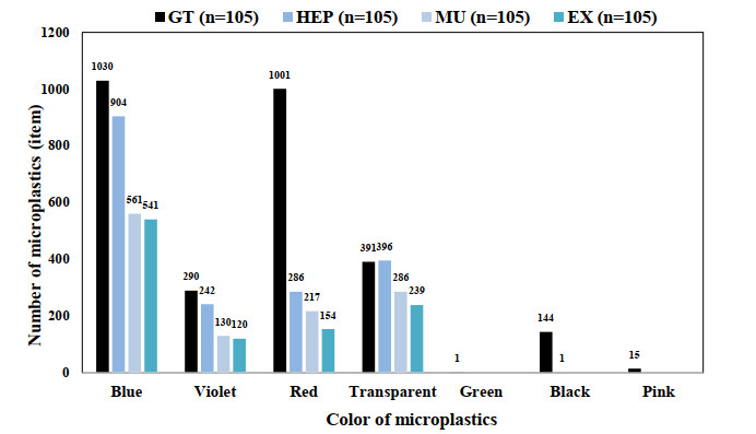
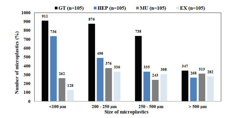
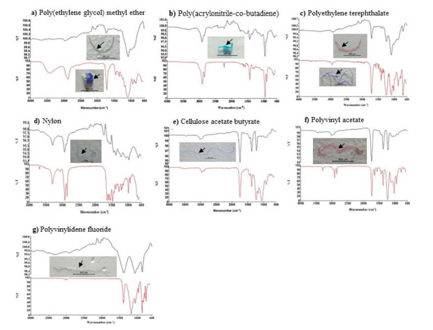
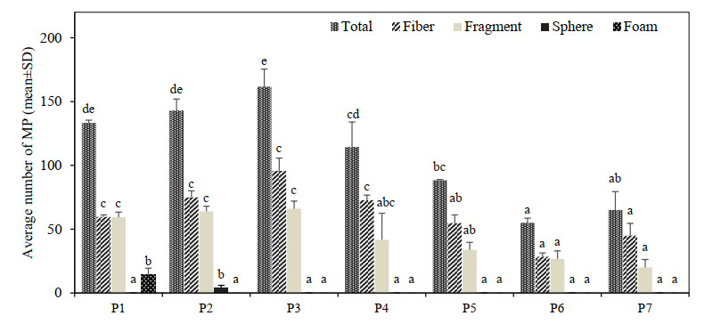
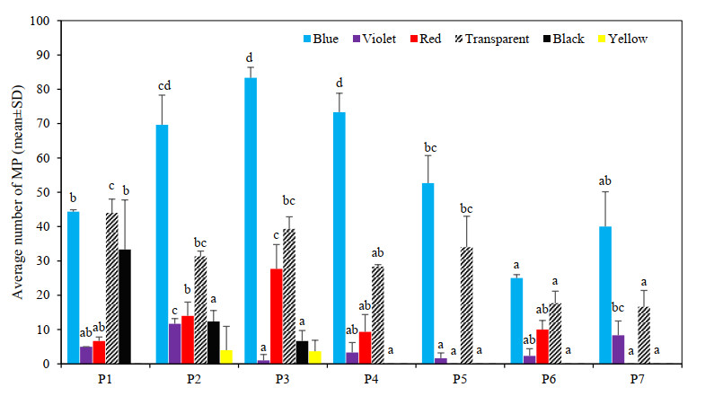
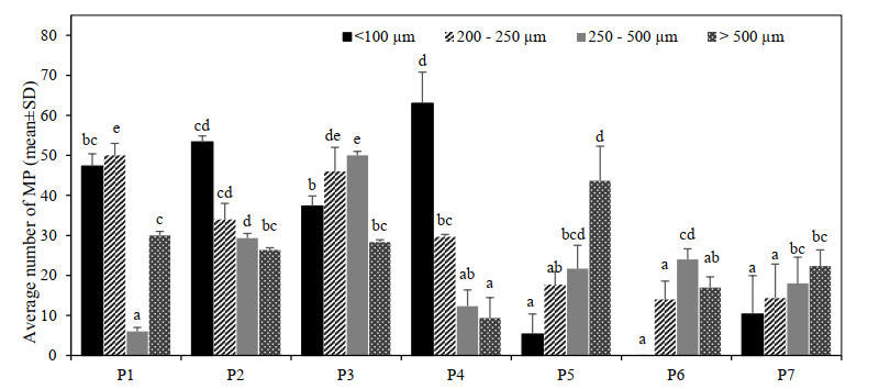
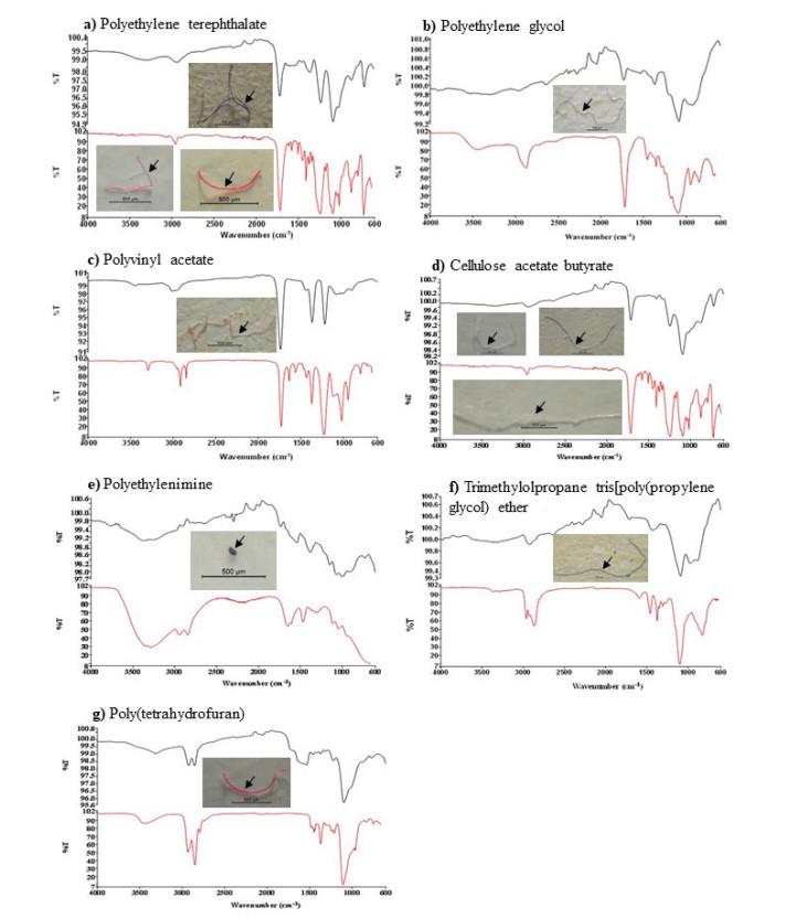
The presence of microplastics in commercially important seafood species is a new issue of food safety concern. Although plastic debris has been found in the gastrointestinal tracts of several species, the prevalence of microplastics in edible shrimp tissues in Thailand has not yet been established. For the first time, the gastrointestinal tract (GT), heptapancreas (HEP), muscle (MU) and exoskeleton (EX) of farmed white leg shrimp (Litopenaeus vannamei) from commercial aquaculture facilities in Nakhon Pathom Province, Thailand, were analyzed for microplastics (MPs). The number of MP items per tissue was 27.36±2.28 in the GT, 17.42±0.90 in the HEP, 11.37±0.60 in the MU and 10.04±0.52 in the EX. MP concentrations were 137.78±16.48, 16.31±1.87, 1.69±0.13 and 4.37±0.27 items/gram (ww) in the GT, HEP, MU and EX, respectively. Microplastics ranged in size from < 100 to 200–250 μm, with fragment-shape (62.07%), fibers (37.31%) and blue (43.69%) was the most common. The most frequently found polymers in shrimp tissue organs and pond water were polyethylene terephthalate (PET), polyvinyl acetate (PVAc) and cellulose acetate butyrate (CAB). Shrimp consumption (excluding GT and EX) was calculated as 28.79 items/shrimp/person/day using Thailand's consumption of shrimp, MP abundance and shrimp consumption. The results of the study can be used as background data for future biomonitoring of microplastics in shrimp species that are significant from an ecological and commercial perspective. MP abundance in farmed L. vannamei may be related to feeding habits and the source of MPs could come from the aquaculture facilities operations.

| [1] |
Benson NU, Bassey DE, Palanisami T (2021) COVID pollution: impact of COVID-19 pandemic on global plastic waste footprint. Heliyon 7: e06343. https://doi:10.1016/j.heliyon.2021.e06343 doi: 10.1016/j.heliyon.2021.e06343

|
| [2] |
Jabeen K, Su L, Li J, et al. (2017) Microplastics and mesoplastics in fish from coastal and fresh waters of China. Environ Pollut 221: 141–149. https://doi.org/10.1016/j.envpol.2016.11.055 doi: 10.1016/j.envpol.2016.11.055
|
| [3] | Frias J, Pagter E, Nash R, et al. (2018) Standardised protocol for monitoring microplastics in sediments. Deliverable D4.2. BASEMAN. Microplastic analyses in European waters: JPI Oceans. https://doi.org/10.13140/RG.2.2.36256.89601/1 |
| [4] |
Hanachi P, Karbalaei S, Walker TR, et al. (2019) Abundance and properties of microplastics found in commercial fish meal and cultured common carp (Cyprinus carpio). Environ Sci Pollut Res 26: 23777–23787. https://doi.org/10.1007/s11356-019-05637-6 doi: 10.1007/s11356-019-05637-6
|
| [5] |
Herrera A, Ŝtindlová A, Martínez I, et al. (2019) Microplastic ingestion by Atlantic chub mackerel (Scomber colias) in the Canary Islands coast. Mar Pollut Bull 139: 127–135. https://doi.org/10.1016/j.marpolbul.2018.12.022 doi: 10.1016/j.marpolbul.2018.12.022
|
| [6] |
Hossain MS, Sobhan F, Uddin MN, et al. (2019) Microplastics in fishes from the Northern Bay of Bengal. Sci Total Environ 690: 821–830. https://doi.org/10.1016/j.scitotenv.2019.07.065 doi: 10.1016/j.scitotenv.2019.07.065
|
| [7] |
Amin RM, Sohaimi ES, Anuar ST, et al. (2020) Microplastic ingestion by zooplankton in Terengganu coastal waters, southern South China Sea. Mar Pollut Bull 150: 110616. https://doi.org/10.1016/j.marpolbul.2019.110616 doi: 10.1016/j.marpolbul.2019.110616
|
| [8] |
Filgueiras AV, Preciado I, Cartón A, et al. (2020) Microplastic ingestion by pelagic and benthic fish and diet composition: a case study in the NW Iberian shelf. Mar Pollut Bull 160: 111623. https://doi.org/10.1016/j.marpolbul.2020.111623 doi: 10.1016/j.marpolbul.2020.111623
|
| [9] |
Kor K, Ghazilou A, Ershadifar H (2020) Microplastic pollution in the littoral sediments of the northern part of the Oman Sea. Mar Pollut Bull 155: 111166. https://doi.org/10.1016/j.marpolbul.2020.111166 doi: 10.1016/j.marpolbul.2020.111166
|
| [10] |
Barboza LGA, Lopes C, Oliveira P, et al. (2020) Microplastics in wild fish from North East Atlantic Ocean and its potential for causing neurotoxic effects, lipid oxidative damage, and human health risks associated with ingestion exposure. Sci Total Environ 717: 134625. https://doi.org/10.1016/j.scitotenv.2019.134625 doi: 10.1016/j.scitotenv.2019.134625
|
| [11] |
Zakeri M, Naji A, Akbarzadeh A, et al. (2020) Microplastic ingestion in important commercial fish in the southern Caspian Sea. Mar Pollut Bull 160: 111598. https://doi.org/10.1016/j.marpolbul.2020.111598. doi: 10.1016/j.marpolbul.2020.111598
|
| [12] |
Kolandhasamy P, Su L, Li J, et al. (2018) Adherence of microplastics to soft tissue of mussels: a novel way to uptake microplastics beyond ingestion. Sci Total Environ 610–611: 635–640. https://doi.org/10.1016/j.scitotenv.2017.08.053 doi: 10.1016/j.scitotenv.2017.08.053
|
| [13] |
Baalkhuyur FM, Qurban MA, Panickan P, et al. (2020) Microplastics in fishes of commercial and ecological importance from the Western Arabian Gulf. Mar Pollut Bull 152: 110920. https://doi.org/10.1016/j.marpolbul.2020.110920 doi: 10.1016/j.marpolbul.2020.110920
|
| [14] |
Li B, Su L, Zhang H, et al. (2020) Microplastics in fishes and their living environments surrounding a plastic production area. Sci Total Environ 727: 138662. https://doi.org/10.1016/j.scitotenv.2020.138662. doi: 10.1016/j.scitotenv.2020.138662
|
| [15] |
Claessens M, Van Cauwenberghe L, Vandegehuchte MB, et al. (2013) New techniques for the detection of microplastics in sediments and field collected organisms. Mar Pollut Bull 70: 227–233. https://doi.org/10.1016/j.marpolbul.2013.03.009 doi: 10.1016/j.marpolbul.2013.03.009
|
| [16] |
Carbery M, O'Connor W, Palanisami T (2018) Trophic transfer of microplastics and mixed contaminants in the marine food web and implications for human health. Environ Int 115: 400–409. https://doi.org/10.1016/j.envint.2018.03.007 doi: 10.1016/j.envint.2018.03.007
|
| [17] |
Wang Q, Zhu X, Hou C, et al. (2021) Microplastic uptake in commercial fishes from the Bohai Sea, China. Chemosphere 263: 127962. https://doi.org/10.1016/j.Chemosphere.2020.127962 doi: 10.1016/j.Chemosphere.2020.127962
|
| [18] |
Lindeque PK, Cole M, Coppock RL, et al. (2020) Are we underestimating microplastic abundance in the marine environment? A comparison of microplastic capture with nets of different mesh-size. Environ Pollut 265: 114721. https://doi.org/10.1016/j.envpol.2020.114721 doi: 10.1016/j.envpol.2020.114721
|
| [19] |
Sfriso AA, Tomio Y, Rosso B, et al. (2020) Microplastic accumulation in benthic invertebrates in Terra Nova Bay (Ross Sea, Antarctica). Environ Int 137: 10558. https://doi.org/10.1016/j.envint.2020.105587 doi: 10.1016/j.envint.2020.105587
|
| [20] |
Daniel DB, Ashraf PM, Thomas SN (2020) Abundance, characteristics and seasonal variation of microplastics in Indian white shrimps (Fenneropenaeus Indicus) from coastal waters off Cochin, Kerala, India. Sci Total Environ 737: 139839. https://doi.org/10.1016/j.scitotenv.2020.139839 doi: 10.1016/j.scitotenv.2020.139839
|
| [21] |
Devriese LI, van der Meulen MD, Maes T, et al. (2015) Microplastic contamination in brown shrimp (Crangon crangon, Linnaeus 1758) from coastal waters of the southern North Sea and channel area. Mar Pollut Bull 98: 179–187. https://doi.org/10.1016/j.marpolbul.2015.06.051 doi: 10.1016/j.marpolbul.2015.06.051
|
| [22] |
Hossain MS, Rahman MS, Uddin MN, et al. (2020) Microplastic contamination in Penaeid shrimp from the Northern Bay of Bengal. Chemosphere 238: 124688. https://doi.org/10.1016/j.chemosphere.2019.124688 doi: 10.1016/j.chemosphere.2019.124688
|
| [23] |
Gray AD, Weinstein JE (2017) Size- and shape-dependent effects of microplastic particles on adult daggerblade grass shrimp (Palaemonetes pugio). Environ Toxicol 36: 3074–3080. https://doi.org/10.1002/etc.3881 doi: 10.1002/etc.3881
|
| [24] |
Qu X, Su L, Li H, et al. (2018) Assessing the relationship between the abundance and properties of microplastics in water and in mussels. Sci Total Environ 621: 679–686. https://doi.org/10.1016/j.scitotenv.2017.11.284 doi: 10.1016/j.scitotenv.2017.11.284
|
| [25] |
Phuong NN, Duong TT, Le TPQ, et al (2022) Microplastics in Asian freshwater ecosystems: current knowledge and perspectives. Sci Total Environ 808: 151989. https://doi:10.1016/j.scitotenv.2021.151989 doi: 10.1016/j.scitotenv.2021.151989
|
| [26] | Masura J, Baker J, Foster G, et al. (2015) Laboratory Methods for the Analysis of Microplastics in the Marine Environment: Recommendations for Quantifying Synthetic Particles in Waters and Sediments. Maryland, USA: NOAA Marine Debris Division. |
| [27] |
Avio CG, Gorbi S, Regoli F (2015) Experimental development of a new protocol for extraction and characterization of microplastics in fish tissues: first observations in commercial species from Adriatic Sea. Mar Environl Res 111: 18–26. https://doi.org/10.1016/j.marenvres.2015.06.014. doi: 10.1016/j.marenvres.2015.06.014
|
| [28] |
Zhang K, Su J, Xiong X, et al. (2016) Microplastic pollution of lakeshore sediments from remote lakes in Tibet plateau, China. Environ Pollut 219: 450–455. https://doi.org/10.1016/j.envpol.2016.05.048 doi: 10.1016/j.envpol.2016.05.048
|
| [29] |
Hidalgo-Ruz V, Gutow L, Thompson RC, et al. (2012) Microplastics in the marine environment: a review of the methods used for identification and quantification. Environ Sci Technol 46: 3060–3075. https://doi.org/10.1021/es2031505 doi: 10.1021/es2031505
|
| [30] |
Su L, Cai H, Kolandhasamy P, et al. (2018) Using the Asian clam as an indicator of microplastic pollution in freshwater ecosystems. Environ Pollut 234: 347−355. https://doi.org/10.1016/j.envpol.2017.11.075 doi: 10.1016/j.envpol.2017.11.075
|
| [31] |
Bergmann M, Wirzberger V, Krumpen T, et al. (2017) High quantities of microplastic in Arctic deep-sea sediments from the HAUSGARTEN Observatory. Environ Sci Technol 51: 11000–11010. https://doi.org/10.1021/acs.est.7b03331 doi: 10.1021/acs.est.7b03331
|
| [32] |
Smith M, Love DC, Rochman CM, et al. (2018) Microplastics in seafood and the implications for human health. Curr Environ Health Rep 5: 375–386. https://doi.org/10.1007/s40572-018-0206-z doi: 10.1007/s40572-018-0206-z
|
| [33] |
Hossain MS, Rahman MS, Uddin MN, et al. (2020) Microplastic contamination in Penaeid shrimp from the Northern Bay of Bengal. Chemosphere 238: 124688. https://doi.org/10.1016/j.chemosphere.2019.124688 doi: 10.1016/j.chemosphere.2019.124688
|
| [34] |
Gurjar UR, Xavier M, Nayak BB, et al. (2021) Microplastics in shrimps: a study from the trawling grounds of north eastern part of Arabian Sea. Environ Sci Pollut Res 28: 48494–48504. https://doi.org/10.1007/s11356-021-14121-z doi: 10.1007/s11356-021-14121-z
|
| [35] |
Wang S, Zhang C, Pan Z, et al. (2020) Microplastics in wild freshwater fish of different feeding habits from Beijiang and Pearl River Delta regions, south China. Chemosphere 258: 127345. https://doi.org/10.1016/j.chemosphere.2020.127345 doi: 10.1016/j.chemosphere.2020.127345
|
| [36] |
Curren E, Leaw CP, Lim PT, et al. (2020) Evidence of marine microplastics in commercially harvested seafood. Front Bioeng Biotechnol 8: 562760. https://doi.org/10.3389/fbioe.2020.562760 doi: 10.3389/fbioe.2020.562760
|
| [37] |
Reunura T, Prommi TO (2022) Detection of microplastics in Litopenaeus vannamei (Penaeidae) and Macrobrachium rosenbergii (Palaemonidae) in cultured pond. PeerJ 10: e12916. https://doi.org/10.7717/peerj.12916 doi: 10.7717/peerj.12916
|
| [38] |
Yoon H, Park B, Rim J, et al. (2022) Detection of microplastics by various types of whiteleg shrimp (Litopenaeus vannamei) in the Korean Sea. Separations 9: 332. https://doi.org/10.3390/separations9110332 doi: 10.3390/separations9110332
|
| [39] |
Barrows A, Cathey SE, Petersen CW (2018) Marine environment microfiber contamination: global patterns and the diversity of microparticle origins. Environ Pollut 237: 275–284. https://doi.org/10.1016/j.envpol.2018.02.062 doi: 10.1016/j.envpol.2018.02.062
|
| [40] |
Capparelli MV, Molinero J, Moulatlet GM, et al. (2021) Microplastics in rivers and coastal waters of the province of Esmeraldas, Ecuador. Mar Pollut Bull 173: 113067. https://doi.org/10.1016/j.marpolbul.2021.113067 doi: 10.1016/j.marpolbul.2021.113067
|
| [41] |
Valencia-Castañeda G, Ruiz-Fernández AC, Frías-Espericueta MG, et al. (2022) Microplastics in the tissues of commercial semi-intensive shrimp pond-farmed Litopenaeus vannamei from the Gulf of California ecoregion. Chemosphere 297: 134194. https://doi.org/10.1016/j.chemosphere.2022.134194 doi: 10.1016/j.chemosphere.2022.134194
|
| [42] |
Wu F, Wang Y, Leung JYS, et al. (2020) Accumulation of microplastics in typical commercial aquatic species: a case study at a productive aquaculture site in China. Sci Total Environ 708: 135432. https://doi.org/10.1016/j.scitotenv.2019.135432 doi: 10.1016/j.scitotenv.2019.135432
|
| [43] |
Keshavarzifard M, Vazirzadeh A, Sharifnia M (2021) Occurrence and characterization of microplastics in white shrimp, Metapenaeus affinis, living in a habitat highly affected by anthropogenic pressures, northwest Persian Gulf. Mar Pollut Bull 169: 112581. https://doi.org/10.1016/j.marpolbul.2021.112581 doi: 10.1016/j.marpolbul.2021.112581
|
| [44] |
Valencia-Castañeda G, Ruiz-Fernández AC, Frías-Espericueta MG, et al. (2022) Microplastics in the tissues of commercial semi-intensive shrimp pond-farmed Litopenaeus vannamei from the Gulf of California ecoregion. Chemosphere 297: 134194. https://doi.org/10.1016/j.chemosphere.2022.134194 doi: 10.1016/j.chemosphere.2022.134194
|
| [45] |
Weinstein JE, Crocker BK, Gray AD (2016) From macroplastic to microplastic: Degradation of high-density polyethylene, polypropylene, and polystyrene in a salt marsh habitat. Environ Toxicol Chem 35: 1632–1640. https://doi.org/10.1002/etc.3432 doi: 10.1002/etc.3432
|
| [46] | Dall W, Hill BJ, Rothlisberg PC, et al. (1990) The Biology of the Penaeidae. Academic Press, San Diego, USA. |
| [47] |
Yan MT, Li WX, Chen XF, He YH, Zhang XY, Gong H (2021) A preliminary study of the association between colonization of microorganism on microplastics and intestinal microbiota in shrimp under natural conditions. J Hazard Mater 408: 124882. https://doi.org/10.1016/j.jhazmat.2020.124882 doi: 10.1016/j.jhazmat.2020.124882
|
| [48] |
Keteles KA, Fleeger JW (2001) The contribution of ecdysis to the fate of copper, zinc and cadmium in grass shrimp, Palaemonetes pugio Holthius. Mar Pollut Bull 42: 1397–1402. https://doi.org/10.1016/S0025-326X(01)00172-2 doi: 10.1016/S0025-326X(01)00172-2
|
| [49] |
Duan Y, Xiong D, Wang Y, et al. (2021) Toxicological effects of microplastics in Litopenaeus vannamei as indicated by an integrated microbiome, proteomic and metabolomic approach. Sci Total Environ 761: 43311. https://doi.org/10.1016/j.scitotenv.2020.143311 doi: 10.1016/j.scitotenv.2020.143311
|
| [50] |
Hsieh SL, Wu YC, Xu RQ, et al. (2021) Effect of polyethylene microplastics on oxidative stress and histopathology damages in Litopenaeus vannamei. Environ Pollut 288: 117880. https://doi.org/10.1016/j.envpol.2021.117800 doi: 10.1016/j.envpol.2021.117800
|
| [51] | Barboza LGA, Frias JPGL, Booth AM, et al. (2019) Microplastics Pollution in the Marine Environment v. 3. In: Sheppard C (Ed.), World Seas: An Environmental Evaluation. Volume Ⅲ: Ecological Issues and Environmental Impacts. 2ed. Academic Press (Elsevier), London, pp. 329–351. |
| [52] |
Karami A, Golieskardi A, Choo CK, et al. (2018) Microplastic and mesoplastic contamination in canned sardines and sprats. Sci Total Environ 612: 1380–1386. https://doi.org/10.1016/j.scitotenv.2017.09.005 doi: 10.1016/j.scitotenv.2017.09.005
|
| [53] |
Wright SL, Kelly FJ (2017) Plastic and human health: a micro issue? Environ. Sci. Technol. 51: 6634–6647. https://doi.org/10.1021/acs.est.7b00423 doi: 10.1021/acs.est.7b00423
|
| [54] |
Volkheimer G (1977) Persorption of particles: physiology and pharmacology. Adv Pharmacol Chemother 14: 163–187. https://doi.org/10.1016/s1054-3589(08)60188-x doi: 10.1016/s1054-3589(08)60188-x
|
| [55] |
Collard F, Gilbert B, Compère P, et al. (2017) Microplastics in livers of European anchovies (Engraulis encrasicolus, L.). Environ Pollut 229: 1000–1005. https://doi.org/10.1016/j.envpol.2017.07.089 doi: 10.1016/j.envpol.2017.07.089
|
| [56] |
Jovanović B, Gökdağ K, Güven O, et al. (2018) Virgin microplastics are not causing imminent harm to fish after dietary exposure. Mar Pollut Bull 130: 123–131. https://doi.org/10.1016/j.marpolbul.2018.03.016 doi: 10.1016/j.marpolbul.2018.03.016
|
| [57] | FAO. The State of World Fisheries and Aquaculture (2020) Sustainability in Action; FAO: Rome, Italy. |
| [58] |
Barboza LGA, Vethaak AD, Lavorante BR, et al. (2018) Marine microplastic debris: An emerging issue for food security, food safety and human health. Mar Pollut Bull 133: 336–348. https://doi.org/10.1016/j.marpolbul.2018.05.047 doi: 10.1016/j.marpolbul.2018.05.047
|
| [59] |
Kim IS, Chae DH, Kim SK, et al. (2015) Factors influencing the spatial variation of microplastics on high-tidal coastal beaches in Korea. Arch Environ Contam Toxicol 69: 299–309. https://doi.org/10.1007/s00244-015-0155-6 doi: 10.1007/s00244-015-0155-6
|
| [60] |
Beer S, Garm A, Huwer B, et al. (2018) No increase in marine microplastic concentration over the last three decades - a case study from the Baltic Sea. Sci Total Environ 621: 1272–1279. https://doi.org/10.1016/j.scitotenv.2017.10.101 doi: 10.1016/j.scitotenv.2017.10.101
|
| [61] |
Zhu L, Bai H, Chen B, et al. (2018) Microplastic pollution in North Yellow Sea, China: observations on occurrence, distribution and identification. Sci Total Environ 636: 20–29. https://doi.org/10.1016/j.scitotenv.2018.04.182 doi: 10.1016/j.scitotenv.2018.04.182
|
| [62] |
Cheung PK, Fok L (2016) Evidence of microbeads from personal care product contaminating the sea. Mar Pollut Bull 109: 582–585. https://doi.org/10.1016/j.marpolbul.2016.05.046 doi: 10.1016/j.marpolbul.2016.05.046
|
| [63] |
Browne MA, Crump P, Niven SJ, et al. (2011) Accumulation of microplastic on shorelines worldwide: sources and sinks. Environ Sci Technol 45: 9175–9179. https://doi.org/10.1021/es201811s doi: 10.1021/es201811s
|
| [64] |
Qiu Q, Peng J, Yu X, et al. (2015) Occurrence of microplastics in the coastal marine environment: first observation on sediment of China. Mar Pollut Bull 98: 274–280. https://doi.org/10.1016/j.marpolbul.2015.07.028 doi: 10.1016/j.marpolbul.2015.07.028
|
| [65] |
Liu T, Zhao Y, Zhu M, et al. (2020) Seasonal variation of micro and meso-plastics in the seawater of Jiaozhou Bay, the Yellow Sea. Mar Pollut Bull 152: 110922. https://doi.org/10.1016/j.marpolbul.2020.110922 doi: 10.1016/j.marpolbul.2020.110922
|
Figures(12) / Tables(5)

Akekawat Vitheepradit, Taeng-On Prommi. Microplastics in surface water and tissue of white leg shrimp, Litopenaeus vannamei, in a cultured pond in Nakhon Pathom Province, Central Thailand[J]. AIMS Environmental Science, 2023, 10(4): 478-503. doi: 10.3934/environsci.2023027


 DownLoad: