The effects of climate and soil properties on the magnitude of the visual soil quality indicators: a logistic regression approach

Fernando Teixeira; Fernando Teixeira

doi:10.3934/geosci.2023027

AIMS Geosciences

2023, Volume 9, Issue 3: 492-512. doi: 10.3934/geosci.2023027

Previous Article Next Article

Research article Special Issues

The effects of climate and soil properties on the magnitude of the visual soil quality indicators: a logistic regression approach

Fernando Teixeira ^,

MED–Mediterranean Institute for Agriculture, Environment and Development, Institute for Advanced Studies and Research, Universidade de évora, Pólo da Mitra, Ap. 94, 7006-554 évora, Portugal

Received: 30 March 2023 Revised: 12 June 2023 Accepted: 03 July 2023 Published: 13 July 2023

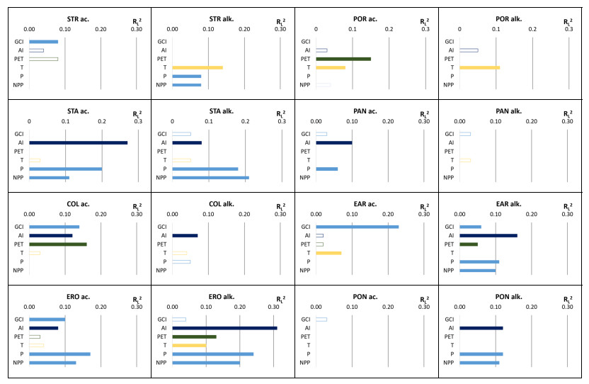
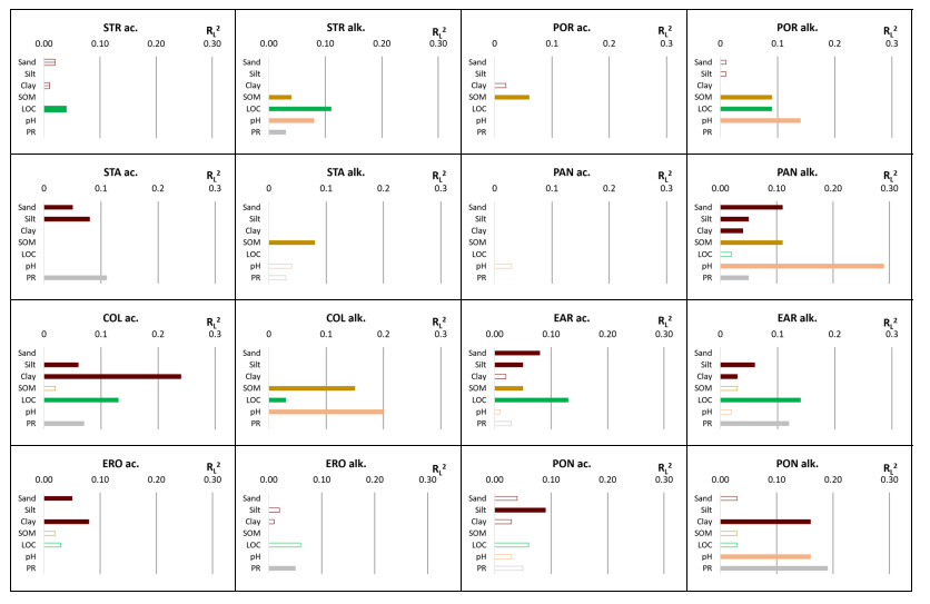
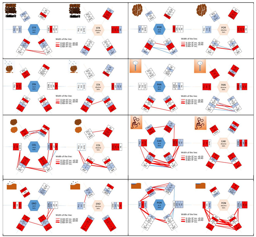
Understanding how different climates and soil properties affect the soil processes requires quantifying these effects. Visual soil quality indicators have been proposed to assess the robustness of the soil processes and infer their ability to function. The scores of the visual soil quality indicators covary with climate features and soil properties, and their magnitude is different in acid-to-neutral and alkaline soils. These variables show collinearities and interactions, and the assessment of the individual effect of each variable on the scores of the visual indicators and the selection of the best set of explanatory variables can only be made with a definite set of variables. Logistic regression was used to calculate the effects of six climate variables and four soil properties, and their interactions, on the scores of eight visual soil quality indicators. Simple models featuring climate and soil variables explained a substantial part of the variation of the visual indicators. Models were fitted for each visual indicator for acid-to-neutral and alkaline soils. The sample size needed was calculated, and the method and its validity were discussed. For two possible outcomes, the sample size using the events per variable (EPV) criterium ranges between 62 and 183 observations, while using one variable and a variance inflation factor, it ranges between 22 and 234. Except for the model of soil structure and consistency for acid-to-neutral soils, with a C statistic of 0.67, all others had acceptable to excellent discrimination. The models built are adequate, for example, for the large-scale spatial outline of the soil health indices, to couple with soil morphological-dependent pedotransfer functions, and so on. Future models should consider (test) other explanatory variables: other climate variables and indices, other soil properties and soil management practices.

Keywords:

New Zealand visual soil assessment method,
VSA,
logistic regression,
models,
interactions,
climate,
soil properties,
soil reaction

Citation: Fernando Teixeira. The effects of climate and soil properties on the magnitude of the visual soil quality indicators: a logistic regression approach[J]. AIMS Geosciences, 2023, 9(3): 492-512. doi: 10.3934/geosci.2023027

Related Papers:

[1]	Bandar Bin-Mohsin, Muhammad Uzair Awan, Muhammad Zakria Javed, Artion Kashuri, Muhammad Aslam Noor . Fractional integral estimations pertaining to generalized ${\gamma}$ -convex functions involving Raina's function and applications. AIMS Mathematics, 2022, 7(8): 13633-13663. doi: 10.3934/math.2022752
[2]	Thongchai Botmart, Soubhagya Kumar Sahoo, Bibhakar Kodamasingh, Muhammad Amer Latif, Fahd Jarad, Artion Kashuri . Certain midpoint-type Fejér and Hermite-Hadamard inclusions involving fractional integrals with an exponential function in kernel. AIMS Mathematics, 2023, 8(3): 5616-5638. doi: 10.3934/math.2023283
[3]	Shahid Mubeen, Rana Safdar Ali, Iqra Nayab, Gauhar Rahman, Kottakkaran Sooppy Nisar, Dumitru Baleanu . Some generalized fractional integral inequalities with nonsingular function as a kernel. AIMS Mathematics, 2021, 6(4): 3352-3377. doi: 10.3934/math.2021201
[4]	Yu-Pei Lv, Ghulam Farid, Hafsa Yasmeen, Waqas Nazeer, Chahn Yong Jung . Generalization of some fractional versions of Hadamard inequalities via exponentially $(\alpha, h-m)$ -convex functions. AIMS Mathematics, 2021, 6(8): 8978-8999. doi: 10.3934/math.2021521
[5]	Muhammad Imran Asjad, Waqas Ali Faridi, Mohammed M. Al-Shomrani, Abdullahi Yusuf . The generalization of Hermite-Hadamard type Inequality with exp-convexity involving non-singular fractional operator. AIMS Mathematics, 2022, 7(4): 7040-7055. doi: 10.3934/math.2022392
[6]	Shuhong Yu, Tingsong Du . Certain inequalities in frame of the left-sided fractional integral operators having exponential kernels. AIMS Mathematics, 2022, 7(3): 4094-4114. doi: 10.3934/math.2022226
[7]	Hu Ge-JiLe, Saima Rashid, Muhammad Aslam Noor, Arshiya Suhail, Yu-Ming Chu . Some unified bounds for exponentially $tgs$ -convex functions governed by conformable fractional operators. AIMS Mathematics, 2020, 5(6): 6108-6123. doi: 10.3934/math.2020392
[8]	Miguel Vivas-Cortez, Muhammad Aamir Ali, Artion Kashuri, Hüseyin Budak . Generalizations of fractional Hermite-Hadamard-Mercer like inequalities for convex functions. AIMS Mathematics, 2021, 6(9): 9397-9421. doi: 10.3934/math.2021546
[9]	Muhammad Tariq, Asif Ali Shaikh, Sotiris K. Ntouyas, Jessada Tariboon . Some novel refinements of Hermite-Hadamard and Pachpatte type integral inequalities involving a generalized preinvex function pertaining to Caputo-Fabrizio fractional integral operator. AIMS Mathematics, 2023, 8(11): 25572-25610. doi: 10.3934/math.20231306
[10]	Artion Kashuri, Rozana Liko, Silvestru Sever Dragomir . New generalized integral inequalities with applications. AIMS Mathematics, 2019, 4(3): 984-996. doi: 10.3934/math.2019.3.984

Abstract

1. Introduction and preliminaries

Fractional calculus has emerged as one of the most important interdisciplinary subjects. In recent past it experienced rapid development and consequently several new generalizations of classical concepts of fractional calculus have been obtained in the literature, for example, see ^[9].

The classical Riemann-Liouville fractional integrals are defined as:

Definition 1.1 (^[9]). Let ${\mathcal{F}}\in L_{1}[a, b]$ . Then the Riemann-Liouville integrals $J_{a^+}^{\alpha}{\mathcal{F}}$ and $J_{b^-}^{\alpha}{\mathcal{F}}$ of order $\alpha > 0$ with $a\geq 0$ are defined by

$\begin{equation*} J_{a^+}^{\alpha}{\mathcal{F}}(x) = \frac{1}{\Gamma(\alpha)}\int\limits_a^x(x-v)^{\alpha-1}{\mathcal{F}}(v){\mathrm{d}}v,\quad x > a, \end{equation*}$

and

$\begin{equation*} J_{b^-}^{\alpha}{\mathcal{F}}(x) = \frac{1}{\Gamma(\alpha)}\int\limits_x^b(v-x)^{\alpha-1}{\mathcal{F}}(v){\mathrm{d}}v,\quad x < b, \end{equation*}$

where

$\begin{align*} \Gamma(x) = \int_0^\infty e^{-v}v^{x-1}{\mathrm{d}}v, \end{align*}$

is the well known Gamma function.

Diaz et al. ^[8] introduced the notion of generalized $k$ -gamma function. The integral form of $\Gamma_{k}$ is given by:

$\begin{equation*} \Gamma_{k}(x) = \int\limits_{0}^{\infty}v^{x-1}e^{-\frac{v^{k}}{k}}{\mathrm{d}}v,\quad \Re(x) > 0. \end{equation*}$

Note that

$\Gamma_{k}(x) = k^{\frac{x}{k}-1}\Gamma\left(\frac{x}{k}\right).$

$k$ -Beta function is defined as:

$\begin{equation*} \beta_{k}(x,y) = \frac{1}{k}\int\limits_{0}^{1}v^{\frac{x}{k}-1}(1-v)^{\frac{x}{k}-1}{\mathrm{d}}v. \end{equation*}$

Obviously

$\beta_{k}(x,y) = \frac{1}{k}\beta\left(\frac{x}{k},\frac{y}{k}\right).$

Sarikaya et al. ^[18] extended the notion of Riemann-Liouville fractional integrals to $k$ -Riemann-Liouville fractional integrals and discussed some of its interesting properties.

To be more precise let ${\mathcal{F}}$ be piecewise continuous on $I^{*} = (0, \infty)$ and integrable on any finite subinterval of $I = [0, \infty]$ . Then for $v > 0$ , we consider $k$ -Riemann-Liouville fractional integral of ${\mathcal{F}}$ of order $\alpha$

$\begin{align*} _kJ_{a}^{\alpha}{\mathcal{F}}(x) = \frac{1}{k\Gamma_{k}(\alpha)}\int\limits_{a}^{x}(x-v)^{\frac{\alpha}{k}-1}{\mathcal{F}}(v){\mathrm{d}}v,\quad x > a,k > 0. \end{align*}$

It has been observed that $k$ -fractional integrals are significant generalizations of classical fractional integrals. For more details, see ^[18].

Ahmad et al. ^[1] defined fractional integral operators with an exponential kernel and obtained corresponding inequalities.

Definition 1.2. Let $\mathcal{F}\in [a, b]$ . The fractional left side integral $\, _{k}\mathcal{I}^{\alpha}_{a^{+}}\mathcal{F}$ and right side integral $\, _{k}\mathcal{I}^{\alpha}_{b^{-}}\mathcal{F}$ of order $\alpha\in(0, 1)$ are defined as follows:

$\mathcal{I}^{\alpha}_{a^{+}}\mathcal{F}(x) = \frac{1}{\alpha}\int\limits_{a}^{x}e^{-\frac{1-\alpha}{\alpha}(x-v)}\mathcal{F}(v){\mathrm{d}}v,\ \ \ \ x > a,$

and

$\mathcal{I}^{\alpha}_{b^{-}}\mathcal{F}(x) = \frac{1}{\alpha}\int\limits_{x}^{b}e^{-\frac{1-\alpha}{\alpha}(v-x)}\mathcal{F}(v){\mathrm{d}}v,\ \ \ \ x < b.$

Using the ideas of ^[1,18], we now introduce the notion of $k$ -fractional integral operators with an exponential kernel.

Definition 1.3. Let $\mathcal{F}\in L[a, b]$ . The $k$ -fractional left side integral $\, _{k}\mathcal{I}^{\alpha}_{a^{+}}\mathcal{F}$ and right side integral $\, _{k}\mathcal{I}^{\alpha}_{b^{-}}\mathcal{F}$ of order $\alpha\in(0, 1)$ for $k > 0$ are defined as follows

$_{k}\mathcal{I}^{\alpha}_{a^{+}}\mathcal{F}(x) = \frac{k}{\alpha}\int\limits_{a}^{x}e^{-\frac{k-\alpha}{\alpha}(x-v)}\mathcal{F}(v){\mathrm{d}}v,\ \ \ \ x > a,$

and

$_{k}\mathcal{I}^{\alpha}_{b^{-}}\mathcal{F}(x) = \frac{k}{\alpha}\int\limits_{x}^{b}e^{-\frac{k-\alpha}{\alpha}(v-x)}\mathcal{F}(v){\mathrm{d}}v,\ \ \ \ x < b.$

It is to be noted that by taking $k \to 1$ in Definition 1.3, we recapture Definition 1.2. Fractional analogues of integral inequalities have a great many applications in numerical quadrature, transform theory, probability, statistical problems etc. Therefore, a significant and rapid development in this field has been noticed, for details, see ^{[2,3,20,24,25]}. Sarikaya et al. ^[19] utilized the concepts of fractional integrals and obtained new fractional refinements of trapezium like inequalities. This article motivated many researchers and as a result several new fractional extensions of classical inequalities have been obtained in the literature, for example, see ^{[1,4,6,7,11,14,15,16,17,18,19,22,23]}. Recently Ahmad et al. ^[1] used fractional integral operators with an exponential kernel and obtained corresponding inequalities. Wu et al. ^[23] derived some new identities and bounds pertaining to fractional integrals with the exponential kernel.

The main motivation of this paper is to derive some new fractional refinements of trapezium like inequalities essentially using the new fractional integral operators with an exponential kernel to $k$ -fractional integral operators with an exponential kernel and the preinvexity property of the functions. In order to establish the significance of our main results, we offer some applications of our main results to means and $q$ -digamma functions. We hope that the ideas and techniques of this paper will inspire interested readers working in the field of inequalities.

Before we proceed further, we now recall some previously known concepts from convex analysis. We first, start with the definition of invex sets.

Definition 1.4 (^[10]). A set $K$ is said to be invex with respect to bifunction $\theta(., .)$ , if

$x+v\theta(y,x)\in K,\,\forall x,y\in K,\,v\in[0,1].$

The preinvexity of the functions is defined as:

Definition 1.5 (^[21]). A function $\mathcal{F}:K\to\mathbb{R}$ is said to be preinvex with respect to bifunction $\theta(., .)$ , if

${\mathcal{F}}(x+v\theta(y,x))\leq(1-v){\mathcal{F}}(x)+vf(y),\,\forall x,y\in K, v\in[0,1].$

In order to obtain some of the main results of the paper, we need the famous condition C, which was introduced by Mohan and Neogy ^[13]. This condition played a vital role in the development of several results involving preinvex functions.

Condition C. Let $\theta:K\times K\to\mathbb{R}^{n}$ . We say that the bifunction $\theta(., .)$ satisfies the condition C, if for any $x, y\in\mathbb{R}^{n}$

1. $\theta(x, x+v\theta(y, x)) = -v\theta(y, x)$ ,

2. $\theta(y, x+v\theta(y, x)) = (1-v)\theta(y, x)$ ,

for all $v\in[0, 1]$ .

Note that for any $x, y\in\mathbb{R}^{n}$ and $v_{1}, v_{2}\in[0, 1]$ and from the condition C, we have, see ^[12]

$\theta(x+v_{2}\theta(y,x),x+v_{1}\theta(y,x)) = (v_{2}-v_{1})\theta(y,x).$

2. Trapezium type inequalities

In this section, we derive some new fractional trapezium type inequalities involving the functions having preinvexity property. For the sake of simplicity, we set $\rho = \frac{k-\alpha}{\alpha}\theta(b, a)$ and $\rho_1 = \frac{1-\alpha}{\alpha}\theta(b, a)$ .

Theorem 2.1. Let $\mathcal{F}:[a, a+\theta(b, a)]\subseteq\mathbb{R}\to\mathbb{R}$ be a positive function with $\theta(b, a) > 0$ and $\mathcal{F}\in L[a, a+\theta(b, a)]$ . Suppose $\mathcal{F}$ is a preinvex function and $\theta(., .)$ satisfies condition C, then

$\begin{align} \mathcal{F}\left(\frac{2a+\theta(b,a)}{2}\right)\leq\frac{k-\alpha}{2k(1-e^{-\rho})}[\,_{k}\mathcal{I}^{\alpha}_{(a)^{+}}\mathcal{F}(a+\theta(b,a))+\,_{k}\mathcal{I}^{\alpha}_{(a+\theta(b,a))^{-}}\mathcal{F}(a)]\leq\frac{\mathcal{F}(a)+\mathcal{F}(b)}{2}. \end{align}$

(2.1)

Proof. By preinvexity of $\mathcal{F}$ , we have for every $x, y\in [a, a+\theta(b, a)]$ with $\lambda = \frac{1}{2}$

$\begin{align*} 2\mathcal{F}\left(x+\frac{\theta(y,x)}{2}\right)\leq[\mathcal{F}(x)+\mathcal{F}(y)], \end{align*}$

with $x = a+v\theta(b, a), y = a+(1-v)\theta(b, a)$ and using the condition C, we have

$\begin{align} &2\mathcal{F}\left(a+v\theta(b,a)+\frac{\theta(a+(1-v)\theta(b,a),a+v\theta(b,a))}{2}\right)\\ & = 2\mathcal{F}\left(a+v\theta(b,a)+\frac{(1-2v)\theta(b,a)}{2}\right)\\ & = 2\mathcal{F}\left(\frac{2a+\theta(b,a)}{2}\right)\\ &\leq\mathcal{F}(a+v\theta(b,a))+\mathcal{F}(a+(1-v)\theta(b,a)). \end{align}$

(2.2)

Multiplying both sides of above inequality by $e^{-\rho v}$ and integrating with respect to $v$ over $[0, 1]$ , we have

$\begin{align*} \frac{2(1-e^{-\rho})}{\rho}\mathcal{F}\left(\frac{2a+\theta(b,a)}{2}\right)&\leq\int\limits^{1}_{0}e^{-\rho v}f(a+v\theta(b,a)){\mathrm{d}}v+\int\limits^{1}_{0}e^{-\rho v}\mathcal{F}(a+(1-v)\theta(b,a)){\mathrm{d}}v\\ & = \frac{1}{\theta(b,a)}\left[\int\limits^{a+\theta(b,a)}_{a}e^{-\rho(\frac{s-a}{\theta(b,a)})}\mathcal{F}(s){\mathrm{d}}s+\int\limits^{a+\theta(b,a)}_{a}e^{-\rho(\frac{a+\theta(b,a)-s}{\theta(b,a)})}\mathcal{F}(s){\mathrm{d}}s\right]\\ & = \frac{\alpha}{k\theta(b,a)}\left[\,_{k}\mathcal{I}^{\alpha}_{(a)^{+}}\mathcal{F}(a+\theta(b,a))+\,_{k}\mathcal{I}^{\alpha}_{(a+\theta(b,a))^{-}}\mathcal{F}(a)\right]. \end{align*}$

As a result, we get

(2.3)

For the proof of second inequality, we note that $\mathcal{F}$ is a preinvex function, so we have

$\begin{align} \mathcal{F}(a+v\theta(b,a))+\mathcal{F}(a+(1-v)\theta(b,a))\leq\mathcal{F}(a)+\mathcal{F}(b). \end{align}$

(2.4)

Multiplying both sides by $e^{-\rho v}$ and integrating with respect to $v$ over $[0, 1]$ , we have

$\begin{align} \frac{\alpha}{k\theta(b,a)}\left[\,_{k}\mathcal{I}^{\alpha}_{(a)^{+}}\mathcal{F}(a+\theta(b,a))+\,_{k}\mathcal{I}^{\alpha}_{(a+\theta(b,a))^{-}}\mathcal{F}(a)\right]\leq\frac{1-e^{-\rho}}{\rho}[\mathcal{F}(a)+\mathcal{F}(b)], \end{align}$

(2.5)

Combining (2.3) and (2.5) completes the proof.

Theorem 2.2. Let $\mathcal{F}:[a, a+\theta(b, a)]\subseteq\mathbb{R}\to\mathbb{R}$ be a positive and preinvex function with $\theta(b, a) > 0$ and $\mathcal{F}\in L[a, a+\theta(b, a)]$ . Let $W$ be a non-negative, integrable and symmetric with respect to $\frac{2a+\theta(b, a)}{2}$ , then using the condition C, we have

$\begin{align} &\mathcal{F}\left(\frac{2a+\theta(b,a)}{2}\right)[\,_{k}\mathcal{I}^{\alpha}_{(a)^{+}}\mathcal{W}(a+\theta(b,a))+\,_{k}\mathcal{I}^{\alpha}_{(a+\theta(b,a))^{-}}\mathcal{W}(a)]\\ &\leq\,_{k}\mathcal{I}^{\alpha}_{(a)^{+}}\mathcal{(FW)}(a+\theta(b,a))+\,_{k}\mathcal{I}^{\alpha}_{(a+\theta(b,a))^{-}}\mathcal{(FW)}(a)\\ &\leq\frac{\mathcal{F}(a)+\mathcal{F}(b)}{2}[\,_{k}\mathcal{I}^{\alpha}_{(a)^{+}}\mathcal{W}(a+\theta(b,a))+\,_{k}\mathcal{I}^{\alpha}_{(a+\theta(b,a))^{-}}\mathcal{W}(a)]. \end{align}$

(2.6)

Proof. Since $\mathcal{F}$ is preinvex function on $L[a, a+\theta(b, a)]$ , so multiplying inequality (2.2) by

$\begin{align} e^{-\rho v}\mathcal{W}(a+v\theta(b,a)), \end{align}$

(2.7)

and then integrating with respect to $v$ over $[0, 1]$ , we get

$\begin{align*} &2\mathcal{F}\left(\frac{2a+\theta(b,a)}{2}\right)\int\limits_{0}^{1}e^{-\rho v}\mathcal{W}(a+v\theta(b,a)){\mathrm{d}}v\\ &\leq\int\limits^{1}_{0}e^{-\rho v}\mathcal{W}(a+v\theta(b,a))\mathcal{F}(a+v\theta(b,a)){\mathrm{d}}v +\int\limits^{1}_{0}e^{-\rho v}\mathcal{W}(a+v\theta(b,a))\mathcal{F}(a+(1-v)\theta(b,a)){\mathrm{d}}v\\ & = \int\limits^{1}_{0}e^{-\rho v}\mathcal{W}(a+v\theta(b,a))\mathcal{F}(a+v\theta(b,a)){\mathrm{d}}v+\int\limits^{1}_{0}e^{-\rho v}\mathcal{W}(a+(1-v)\theta(b,a))\mathcal{F}(a+(1-v)\theta(b,a)){\mathrm{d}}v\\ & = \frac{1}{\theta(b,a)}\left[\int\limits^{a+\theta(b,a)}_{a}e^{-\rho(\frac{s-a}{\theta(b,a)})}\mathcal{F}(s)\mathcal{W}(s){\mathrm{d}}s+\int\limits^{a+\theta(b,a)}_{a}e^{-\rho(\frac{a+\theta(b,a)-s}{\theta(b,a)})}\mathcal{F}(s)\mathcal{W}(s){\mathrm{d}}s\right]\\ & = \frac{\alpha}{k\theta{(b,a)}}[\,_{k}\mathcal{I}^{\alpha}_{(a)^{+}}\mathcal{(FW)}(a+\theta(b,a))+\,_{k}\mathcal{I}^{\alpha}_{(a+\theta(b,a))^{-}}\mathcal{(FW)}(a)]. \end{align*}$

Thus

$\begin{align*} &2\mathcal{F}\left(\frac{2a+\theta(b,a)}{2}\right)\int\limits_{0}^{1}e^{-\rho v}\mathcal{W}(a+v\theta(b,a)){\mathrm{d}}v\\ &\leq\frac{\alpha}{k\theta{(b,a)}}[\,_{k}\mathcal{I}^{\alpha}_{(a)^{+}}\mathcal{FW}(a+\theta(b,a))+\,_{k}\mathcal{I}^{\alpha}_{(a+\theta(b,a))^{-}}\mathcal{FW}(a)]. \end{align*}$

Since $\mathcal{W}$ is symmetric with respect to $\frac{2a+\theta(b, a)}{2},$ we have

$\,_{k}\mathcal{I}^{\alpha}_{(a)^{+}}\mathcal{W}(a+\theta(b,a)) = \,_{k}\mathcal{I}^{\alpha}_{(a+\theta(b,a))^{-}}\mathcal{W}(a) = \frac{1}{2}[\,_{k}\mathcal{I}^{\alpha}_{(a)^{+}}\mathcal{W}(a+\theta(b,a))+\,_{k}\mathcal{I}^{\alpha}_{(a+\theta(b,a))^{-}}\mathcal{W}(a)].$

Thus we get the left side of inequality (2.6).

For the proof of right side of inequality (2.6), we multiply (2.7) and (2.4) and then integrating the resulting inequality with respect to $v$ over $[0, 1],$ we get the required result.

Theorem 2.3. Let $\mathcal{F, W}:[a, a+\theta(b, a)]\subseteq\mathbb{R}\to\mathbb{R}$ be nonnegative and preinvex function on $L[a, a+\theta(b, a)]$ with $\theta(b, a) > 0$ . If $\theta(., .)$ satisfies condition C, then the following inequalities for the $k$ -fractional integrals with exponential kernel holds:

$\begin{align} &\frac{\alpha}{2k\theta(b,a)}[\,_{k}\mathcal{I}^{\alpha}_{(a)^{+}}\mathcal{(FW)}(a+\theta(b,a))+\,_{k}\mathcal{I}^{\alpha}_{(a+\theta(b,a))^{-}}\mathcal{(FW)}(a)]\\ &\leq M(a,b)\frac{\rho^{2}-2\rho+4-e^{-\rho}(\rho^{2}+2\rho+4)}{2\rho^{3}}+N(a,b)\frac{\rho-2+e^{-\rho}(\rho+2)}{\rho^{3}}, \end{align}$

(2.8)

and

$\begin{align} &2\mathcal{F}\left(\frac{2a+\theta(b,a)}{2}\right)\mathcal{W}\left(\frac{2a+\theta(b,a)}{2}\right)\\ &\leq\frac{k-\alpha}{2k(1-e^{-\rho})}[\,_{k}\mathcal{I}^{\alpha}_{(a)^{+}}\mathcal{FW}(a+\theta(b,a))+\,_{k}\mathcal{I}^{\alpha}_{(a+\theta(b,a))^{-}}\mathcal{FW}(a)]\\ &\leq M(a,b)\frac{\rho-2+e^{-\rho}(\rho+2)}{\rho^{2}(1-e^{-\rho})}+N(a,b)\frac{\rho^{2}-2\rho+4-e^{-\rho}(\rho^{2}+2\rho+4)}{2\rho^{2}(1-e^{-\rho})}, \end{align}$

(2.9)

where

$M(a,b) = \mathcal{F}(a)\mathcal{W}(a)+\mathcal{F}(b)\mathcal{W}(b),$

and

$N(a,b) = \mathcal{F}(a)\mathcal{W}(b)+\mathcal{F}(b)\mathcal{W}(a).$

Proof. Since $\mathcal{F}, \mathcal{W}$ are preinvex functions on $[a, a+\theta(b, a)]$ , then we have

$\begin{align*} \mathcal{F}(a+v\theta(b,a))\mathcal{W}(a+v\theta(b,a))\leq (1-v)^{2}\mathcal{F}(a)\mathcal{W}(a)+v^{2}\mathcal{F}(b)\mathcal{W}(b)+v(1-v)N(a,b), \end{align*}$

and

$\begin{align*} \mathcal{F}(a+(1-v)\theta(b,a))\mathcal{W}(a+(1-v)\theta(b,a))\leq v^{2}\mathcal{F}(a)\mathcal{W}(a)+(1-v)^{2}\mathcal{F}(b)\mathcal{W}(b)+v(1-v)N(a,b). \end{align*}$

Adding above inequalities, we have

$\begin{align*} \mathcal{F}(a+v\theta(b,a))\mathcal{W}(a+v\theta(b,a))&+\mathcal{F}(a+(1-v)\theta(b,a))\mathcal{W}(a+(1-v)\theta(b,a))\\ &\leq(2v^{2}-2v+1)M(a,b)+2v(1-v)N(a,b). \end{align*}$

Multiplying both sides of above inequality by $e^{-\rho v}$ and integrating with respect to $v$ over $[0, 1]$ , we have

$\begin{align*} &\int\limits_{0}^{1}e^{-\rho v}\mathcal{F}(a+v\theta(b,a))\mathcal{W}(a+v\theta(b,a)){\mathrm{d}}v\\ &\quad+\int\limits_{0}^{1}e^{-\rho v}\mathcal{F}(a+(1-v)\theta(b,a))\mathcal{W}(a+(1-v)\theta(b,a)){\mathrm{d}}v\\ &\leq M(a,b)\int\limits_{0}^{1}e^{-\rho v}(2v^{2}-2v+1){\mathrm{d}}v+M(a,b)\int\limits_{0}^{1}e^{-\rho v}2v(1-v){\mathrm{d}}v\\ & = M(a,b)\frac{\rho^{2}-2\rho+4-e^{-\rho}(\rho^{2}+2\rho+4)}{2\rho^{3}}+N(a,b)\frac{\rho-2+e^{-\rho}(\rho+2)}{\rho^{3}}. \end{align*}$

So,

$\begin{align*} &\frac{\alpha}{2k\theta(b,a)}[\,_{k}\mathcal{I}^{\alpha}_{(a)^{+}}\mathcal{(FW)}(a+\theta(b,a))+\,_{k}\mathcal{I}^{\alpha}_{(a+\theta(b,a))^{-}}\mathcal{(FW)}(a)]\\ &\leq M(a,b)\frac{\rho^{2}-2\rho+4-e^{-\rho}(\rho^{2}+2\rho+4)}{2\rho^{3}}+N(a,b)\frac{\rho-2+e^{-\rho}(\rho+2)}{\rho^{3}}. \end{align*}$

For the proof of inequality (2.9), using the preinvexity of $\mathcal{F}, \mathcal{W}$ and condition C, we have

$\begin{align} &\mathcal{F}\left(\frac{2a+\theta(b,a)}{2}\right)\mathcal{W}\left(\frac{2a+\theta(b,a)}{2}\right)\\ & = \mathcal{F}\left(a+(1-v)\theta(b,a)+\frac{1}{2}\theta(a+v\theta(b,a),a+(1-v)\theta(b,a)\right)\\ &\times\mathcal{W}\left(a+(1-v)\theta(b,a)+\frac{1}{2}\theta(a+v\theta(b,a),a+(1-v)\theta(b,a)\right)\\ &\leq\left(\frac{\mathcal{F}(a+v\theta(b,a))+\mathcal{F}(a+(1-v)\theta(b,a))}{2}\right)\left(\frac{\mathcal{W}(a+v\theta(b,a))+\mathcal{W}(a+(1-v)\theta(b,a))}{2}\right)\\ &\leq\frac{\mathcal{F}(a+v\theta(b,a))\mathcal{W}(a+v\theta(b,a))}{4}+\frac{\mathcal{F}(a+(1-v)\theta(b,a))\mathcal{W}(a+(1-v)\theta(b,a))}{4}\\ &+\frac{v(1-v)}{2}M(a,b)+\frac{2v^{2}-2v+1}{4}N(a,b). \end{align}$

(2.10)

Multiplying both sides of inequality (2.10) by $e^{-\rho v}$ and integrating with respect to $v$ over $[0, 1]$ , we get

$\begin{align*} &\frac{1-e^{-\rho}}{\rho}\mathcal{F}\left(\frac{2a+\theta(b,a)}{2}\right)\mathcal{W}\left(\frac{2a+\theta(b,a)}{2}\right)\\ &\leq\int\limits_{0}^{1}e^{-\rho v}\frac{\mathcal{F}(a+v\theta(b,a))\mathcal{W}(a+v\theta(b,a))}{4}{\mathrm{d}}v\\ &+\int\limits_{0}^{1}e^{-\rho v}\frac{\mathcal{F}(a+(1-v)\theta(b,a))\mathcal{W}(a+(1-v)\theta(b,a))}{4}{\mathrm{d}}v\\ &+M(a,b)\int\limits_{0}^{1}e^{-\rho v}\frac{v(1-v)}{2}{\mathrm{d}}v+N(a,b)\int\limits_{0}^{1}e^{-\rho v}\frac{2v^{2}-2v+1}{4}{\mathrm{d}}v, \end{align*}$

which completes the proof.

3. Inequalities involving first and second order differentiable preinvex functions

Lemma 3.1. Assume that $\mathcal{F}:[a, a+\theta(b, a)]\subseteq\mathbb{R}\to\mathbb{R}$ is a differentiable function and $\mathcal{F^{\prime}}\in L[a, a+\theta(b, a)]$ . Then the following equality for the $k$ -fractional integrals with exponential kernel holds:

$\begin{align} R_{ab}& = \frac{\theta(b,a)}{2}\int\limits_{0}^{1}u\mathcal{F^{\prime}}(a+(1-v)\theta(b,a)){\mathrm{d}}v\\ &-\frac{\theta(b,a)}{2(1-e^{-\rho})}\left[\int\limits_{0}^{1}e^{-\rho v}\mathcal{F^{\prime}}(a+(1-v)\theta(b,a)){\mathrm{d}}v-\int\limits_{0}^{1}e^{-\rho(1-v)}\mathcal{F^{\prime}}(a+(1-v)\theta(b,a)){\mathrm{d}}v\right], \end{align}$

(3.1)

where

$\begin{align*} R_{ab} = \frac{k-\alpha}{2k(1-e^{-\rho})}[\,_{k}\mathcal{I}^{\alpha}_{(a)^{+}}\mathcal{F}(a+\theta(b,a))+\,_{k}\mathcal{I}^{\alpha}_{(a+\theta(b,a))^{-}}\mathcal{F}(a)]-\mathcal{F}\left(\frac{2a+\theta(b,a)}{2}\right), \end{align*}$

and

$u = \left\{ \begin{array}{rcl} 1, \ & \mathit{{for}} & 0\leq v\leq\frac{1}{2}, \\\\ -1, & \mathit{{for}} & \frac{1}{2}\leq v\leq1. \end{array}\right.$

Proof. By simple calculations, we have

$\begin{align} &\int\limits_{0}^{1}e^{-\rho v}\mathcal{F^{\prime}}(a+(1-v)\theta(b,a)){\mathrm{d}}v\\ & = -\frac{1}{\theta(b,a)}\left[e^{-\rho v}\mathcal{F}(a+(1-v)\theta(b,a))\bigg|_{0}^{1}+\rho\int\limits_{0}^{1}e^{-\rho v}\mathcal{F}(a+(1-v)\theta(b,a)){\mathrm{d}}v\right]\\ & = -\frac{1}{\theta(b,a)}\left[\mathcal{F}(a+\theta(b,a))-e^{-\rho}\mathcal{F}(a)+\rho\int\limits_{0}^{1}e^{-\rho v}\mathcal{F}(a+(1-v)\theta(b,a)){\mathrm{d}}v\right]\\ & = \frac{1}{\theta(b,a)}\left[\mathcal{F}(a+\theta(b,a))-e^{-\rho}\mathcal{F}(a)-\frac{\rho}{\theta(b,a)}\int\limits_{a}^{a+\theta(b,a)}e^{-\rho \frac{a+\theta(b,a)-s}{\theta(b,a)}}\mathcal{F}(s){\mathrm{d}}s\right]\\ & = \frac{1}{\theta(b,a)}\left[\mathcal{F}(a+\theta(b,a))-e^{-\rho}\mathcal{F}(a)-\frac{k-\alpha}{\alpha}\int\limits_{a}^{a+\theta(b,a)}e^{-\frac{(k-\alpha)}{\alpha} (a+\theta(b,a)-s)}\mathcal{F}(s){\mathrm{d}}s\right]\\ & = \frac{1}{\theta(b,a)}\left[\mathcal{F}(a+\theta(b,a))-e^{-\rho}\mathcal{F}(a)-\frac{k-\alpha}{k}\,_{k}\mathcal{I}^{\alpha}_{(a)^{+}}\mathcal{F}(a+\theta(b,a))\right], \end{align}$

(3.2)

similarly

$\begin{align} &\int\limits_{0}^{1}e^{-\rho (1-v)}\mathcal{F^{\prime}}(a+(1-v)\theta(b,a)){\mathrm{d}}v\\ & = -\frac{1}{\theta(b,a)}\left[e^{-\rho (1-v)}\mathcal{F}(a+(1-v)\theta(b,a))\bigg|_{0}^{1}-\rho\int\limits_{0}^{1}e^{-\rho (1-v)}\mathcal{F}(a+(1-v)\theta(b,a)){\mathrm{d}}v\right]\\ & = -\frac{1}{\theta(b,a)}\left[\mathcal{F}(a)-e^{-\rho}\mathcal{F}(a+\theta(b,a))-\rho\int\limits_{0}^{1}e^{-\rho v}\mathcal{F}(a+(1-v)\theta(b,a)){\mathrm{d}}v\right]\\ & = \frac{1}{\theta(b,a)}\left[e^{-\rho}\mathcal{F}(a+\theta(b,a))-\mathcal{F}(a)+\frac{\rho}{\theta(b,a)}\int\limits_{a}^{a+\theta(b,a)}e^{-\rho \frac{s-a}{\theta(b,a)}}\mathcal{F}(s){\mathrm{d}}s\right]\\ & = \frac{1}{\theta(b,a)}\left[e^{-\rho}\mathcal{F}(a+\theta(b,a))-\mathcal{F}(a)+\frac{k-\alpha}{\alpha}\int\limits_{a}^{a+\theta(b,a)}e^{-\frac{(k-\alpha)}{\alpha} (s-a)}\mathcal{F}(s){\mathrm{d}}s\right]\\ & = \frac{1}{\theta(b,a)}\left[e^{-\rho}\mathcal{F}(a+\theta(b,a))-\mathcal{F}(a)+\frac{k-\alpha}{k}\,_{k}\mathcal{I}^{\alpha}_{(a+\theta(b,a))^{-}}\mathcal{F}(a)\right]. \end{align}$

(3.3)

Also note that

(3.4)

Substituting (3.2), (3.3) and (3.4) in (3.1) completes the proof.

Theorem 3.1. Assume that $\mathcal{F}:[a, a+\theta(b, a)]\subseteq\mathbb{R}\to\mathbb{R}$ is a differentiable function and $\mathcal{F^{\prime}}\in L[a, a+\theta(b, a)]$ and $|\mathcal{F^{\prime}}|$ is preinvex on $[a, a+\theta(b, a)]$ . Then the following inequality for the $k$ -fractional integrals with exponential kernel holds:

$\begin{align*} |R_{ab}|\leq\frac{\theta(b,a)}{2}\left(\frac{1}{2}-\frac{\tanh\left(\frac{\rho}{4}\right)}{\rho}\right)(|\mathcal{F}^{\prime}(a)|+|\mathcal{F}^{\prime}(b)|). \end{align*}$

Proof. Using Lemma 3.1, preinvexity of $|\mathcal{F^{\prime}}|$ and increasing property of exponential function, we have

$\begin{align*} |R_{ab}|& = \left|\frac{\theta(b,a)}{2}\int\limits_{0}^{1}u\mathcal{F^{\prime}}(a+(1-v)\theta(b,a)){\mathrm{d}}v\right.\\ &-\left.\frac{\theta(b,a)}{2(1-e^{-\rho})}\left[\int\limits_{0}^{1}e^{-\rho v}\mathcal{F^{\prime}}(a+(1-v)\theta(b,a)){\mathrm{d}}v-\int\limits_{0}^{1}e^{-\rho(1-v)}\mathcal{F^{\prime}}(a+(1-v)\theta(b,a)){\mathrm{d}}v\right]\right|\\ &\leq\frac{\theta(b,a)}{2(1-e^{-\rho})}\left[\int\limits_{0}^{\frac{1}{2}}\left(1-e^{-\rho}-e^{-\rho v}+e^{-\rho(1-v)}\right)|\mathcal{F^{\prime}}(a+(1-v)\theta(b,a))|{\mathrm{d}}v\right.\\ &\left.-\int\limits_{\frac{1}{2}}^{1}\left(1-e^{-\rho}-e^{-\rho (1-v)}+e^{-\rho v}\right)|\mathcal{F^{\prime}}(a+(1-v)\theta(b,a))|{\mathrm{d}}v\right]\\ &\leq\frac{\theta(b,a)}{2(1-e^{-\rho})}\left[\int\limits_{0}^{\frac{1}{2}}\left(1-e^{-\rho}-e^{-\rho v}+e^{-\rho(1-v)}\right)(v|\mathcal{F^{\prime}}(a)|+(1-v)|\mathcal{F^{\prime}}(b)|){\mathrm{d}}v\right.\\ &\left.-\int\limits_{\frac{1}{2}}^{1}\left(1-e^{-\rho}-e^{-\rho (1-v)}+e^{-\rho v}\right)(v|\mathcal{F^{\prime}}(a)|+(1-v)|\mathcal{F}^{\prime}(b)|){\mathrm{d}}v\right] \\ & = \frac{\theta(b,a)}{2(1-e^{-\rho})}\left[\int\limits_{0}^{\frac{1}{2}}\left(1-e^{-\rho}-e^{-\rho v}+e^{-\rho(1-v)}\right)(v|\mathcal{F^{\prime}}(a)|+(1-v)|\mathcal{F^{\prime}}(b)|){\mathrm{d}}v\right.\\ &\left.-\int\limits_{0}^{\frac{1}{2}}\left(1-e^{-\rho}-e^{-\rho v}+e^{-\rho (1-v)}\right)((1-v)|\mathcal{F^{\prime}}(a)|+v|\mathcal{F}^{\prime}(b)|){\mathrm{d}}v\right]\\ & = \frac{\theta(b,a)}{2(1-e^{-\rho})}\int\limits_{0}^{\frac{1}{2}}\left(1-e^{-\rho}-e^{-\rho v}+e^{-\rho(1-v)}\right)(|\mathcal{F^{\prime}}(a)|+|\mathcal{F^{\prime}}(b)|){\mathrm{d}}v\\ & = \frac{\theta(b,a)}{2(1-e^{-\rho})}\left[\frac{1-e^{-\rho}}{2}-\frac{1}{\rho}(1-e^{\frac{-\rho}{2}})^{2}\right](|\mathcal{F^{\prime}}(a)|+|\mathcal{F^{\prime}}(b)|)\\ & = \frac{\theta(b,a)}{2}\left(\frac{1}{2}-\frac{\tanh\left(\frac{\rho}{4}\right)}{\rho}\right)(|\mathcal{F}^{\prime}(a)|+|\mathcal{F}^{\prime}(b)|), \end{align*}$

which completes the proof.

Lemma 3.2. Assume that $\mathcal{F}:[a, a+\theta(b, a)]\subseteq\mathbb{R}\to\mathbb{R}$ is a differentiable function and $\mathcal{F^{\prime}}\in L[a, a+\theta(b, a)]$ . Then the following equality for the fractional integrals with exponential kernel holds:

$\begin{align} L_{ab} = \frac{\theta(b,a)}{2(1-e^{-\rho})}\left[\int\limits_{0}^{1}e^{-\rho v}\mathcal{F^{\prime}}(a+(1-v)\theta(b,a)){\mathrm{d}}v-\int\limits_{0}^{1}e^{-\rho(1-v)}\mathcal{F^{\prime}}(a+(1-v)\theta(b,a)){\mathrm{d}}v\right], \end{align}$

(3.5)

where

$L_{ab} = \frac{\mathcal{F}(a)+\mathcal{F}(a+\theta(b,a)}{2}-\frac{k-\alpha}{2k(1-e^{-\rho})}[\,_{k}\mathcal{I}^{\alpha}_{(a)^{+}}\mathcal{F}(a+\theta(b,a))+\,_{k}\mathcal{I}^{\alpha}_{(a+\theta(b,a))^{-}}\mathcal{F}(a)].$

Proof. Using 3.2 and 3.3, we get the required result.

Theorem 3.2. Assume that $\mathcal{F}:[a, a+\theta(b, a)]\subseteq\mathbb{R}\to\mathbb{R}$ is a differentiable function and $\mathcal{F^{\prime}}\in L[a, a+\theta(b, a)]$ . If $|\mathcal{F^{\prime}}|$ is preinvex function on $[a, a+\theta(b, a)]$ , then the following inequality for the $k$ -fractional integrals with exponential kernel holds:

$\begin{align*} |L_{ab}|\leq\frac{\theta(b,a)}{2\rho}\tanh\left(\frac{\rho}{4}\right)(|\mathcal{F}^{\prime}(a)|+|\mathcal{F}^{\prime}(b)|). \end{align*}$

Proof. Using Lemma 3.2, preinvexity of $|\mathcal{F^{\prime}}|$ and increasing property of exponential function, we have

$\begin{align*} |L_{ab}|&\leq\frac{\theta(b,a)}{2}\int\limits_{0}^{1}\frac{|e^{-\rho v}-e^{-\rho(1-v)}|}{1-e^{-\rho}}|\mathcal{F^{\prime}}(a+v\theta(b,a))|{\mathrm{d}}v\\ &\leq\frac{\theta(b,a)}{2}\left[\int\limits_{0}^{1}\frac{|e^{-\rho v}-e^{-\rho(1-v)}|}{1-e^{-\rho}}v|\mathcal{F^{\prime}}(a)|{\mathrm{d}}v+\int\limits_{0}^{1}\frac{|e^{-\rho v}-e^{-\rho(1-v)}|}{1-e^{-\rho}}(1-v)|\mathcal{F^{\prime}}(b)|{\mathrm{d}}v\right] \\& = \frac{\theta(b,a)}{2}|\mathcal{F^{\prime}}(a)|\left[\int\limits_{0}^{\frac{1}{2}}\frac{e^{-\rho v}-e^{-\rho(1-v)}}{1-e^{-\rho}}v{\mathrm{d}}v+\int\limits^{1}_{\frac{1}{2}}\frac{e^{-\rho (1-v)}-e^{-\rho v}}{1-e^{-\rho}}v{\mathrm{d}}v\right]\\ &+\frac{\theta(b,a)}{2}|\mathcal{F^{\prime}}(b)|\left[\int\limits_{0}^{\frac{1}{2}}\frac{e^{-\rho v}-e^{-\rho(1-v)}}{1-e^{-\rho}}(1-v){\mathrm{d}}v+\int\limits^{1}_{\frac{1}{2}}\frac{e^{-\rho (1-v)}-e^{-\rho v}}{1-e^{-\rho}}(1-v){\mathrm{d}}v\right]\\ & = \frac{\theta(b,a)}{2\rho}\tanh\left(\frac{\rho}{4}\right)(|\mathcal{F}^{\prime}(a)|+|\mathcal{F}^{\prime}(b)|), \end{align*}$

which completes the proof.

Lemma 3.3. Assume that $\mathcal{F}:[a, a+\theta(b, a)]\subseteq\mathbb{R}\to\mathbb{R}$ is twice differentiable function and $\mathcal{F^{\prime\prime}}\in L[a, a+\theta(b, a)]$ . Then the following equality for the $k$ -fractional integrals with exponential kernel holds:

$\begin{align} L_{ab} = \frac{\theta^{2}(b,a)}{2\rho(1-e^{-\rho})}\int\limits_{0}^{1}\left(1+e^{-\rho}-e^{-\rho v}-e^{-\rho(1-v)}\right)\mathcal{F^{\prime\prime}}(a+(1-v)\theta(b,a)){\mathrm{d}}v. \end{align}$

(3.6)

Proof. Using (3.5) and integration by parts, we have

$\begin{align} &\int\limits_{0}^{1}e^{-\rho v}\mathcal{F}^{\prime}(a+(1-v)\theta(b,a)){\mathrm{d}}v\\ & = -\frac{1}{\rho}\left[e^{-\rho v}\mathcal{F}^{\prime}(a+(1-v)\theta(b,a))\bigg|_{0}^{1}+\theta(b,a)\int\limits_{0}^{1}e^{-\rho v}\mathcal{F}^{\prime\prime}(a+(1-v)\theta(b,a)){\mathrm{d}}v\right]\\ & = -\frac{1}{\rho}\left[e^{-\rho}\mathcal{F}^{\prime}(a)-\mathcal{F}^{\prime}(a+\theta(b,a))+\theta(b,a)\int\limits_{0}^{1}e^{-\rho v}\mathcal{F}^{\prime\prime}(a+(1-v)\theta(b,a)){\mathrm{d}}v\right], \end{align}$

(3.7)

similarly

$\begin{align} &\int\limits_{0}^{1}e^{-\rho (1-v)}\mathcal{F}^{\prime}(a+(1-v)\theta(b,a)){\mathrm{d}}v\\ & = \frac{1}{\rho}\left[e^{-\rho (1-v)}\mathcal{F}^{\prime}(a+(1-v)\theta(b,a))\bigg|_{0}^{1}+\theta(b,a)\int\limits_{0}^{1}e^{-\rho (1-v)}\mathcal{F}^{\prime\prime}(a+(1-v)\theta(b,a)){\mathrm{d}}v\right]\\ & = \frac{1}{\rho}\left[\mathcal{F}^{\prime}(a)-e^{-\rho}\mathcal{F}^{\prime}(a+\theta(b,a))+\theta(b,a)\int\limits_{0}^{1}e^{-\rho (1-v)}\mathcal{F}^{\prime\prime}(a+(1-v)\theta(b,a)){\mathrm{d}}v\right]. \end{align}$

(3.8)

Substituting (3.7) and (3.8) in (3.5), we have

$\begin{align*} L_{ab}& = \frac{\theta(b,a)}{2\rho(1-e^{-\rho})}\left[(1+e^{-\rho})(\mathcal{F}^{\prime}(a+\theta(b,a))-\mathcal{F}^{\prime}(a))\right.\\ &\left.-\theta(b,a)\int\limits_{0}^{1}(e^{-\rho v}+e^{-\rho (1-v)})\mathcal{F}^{\prime\prime}(a+(1-v)\theta(b,a)){\mathrm{d}}v\right]\\ & = \frac{\theta^{2}(b,a)}{2\rho(1-e^{-\rho})}\int\limits_{0}^{1}\left(1+e^{-\rho}-e^{-\rho v}-e^{-\rho(1-v)}\right)\mathcal{F^{\prime\prime}}(a+(1-v)\theta(b,a)){\mathrm{d}}v, \end{align*}$

which completes the proof.

Theorem 3.3. Assume that $\mathcal{F}:[a, a+\theta(b, a)]\subseteq\mathbb{R}\to\mathbb{R}$ is twice differentiable function. If $\mathcal{F^{\prime\prime}}\in L[a, a+\theta(b, a)]$ and $|\mathcal{F^{\prime\prime}}|$ is preinvex on $[a, a+\theta(b, a)]$ , then the following inequality for the $k$ -fractional integrals with exponential kernel holds:

$\begin{align*} |L_{ab}|\leq\frac{\theta^{2}(b,a)}{2\rho(1-e^{-\rho})}\left(\frac{1+e^{-\rho}}{2}-\frac{1-e^{-\rho}}{\rho}\right)(|\mathcal{F}^{\prime\prime}(a)|+|\mathcal{F}^{\prime\prime}(b)|). \end{align*}$

Proof. It is to be noted that

$\begin{align} \int\limits_{0}^{1}\left(1+e^{-\rho}-e^{-\rho v}-e^{-\rho(1-v)}\right)v{\mathrm{d}}v = \frac{1+e^{-\rho}}{2}-\frac{1-e^{-\rho}}{\rho}, \end{align}$

(3.9)

and

$\begin{align} \int\limits_{0}^{1}\left(1+e^{-\rho}-e^{-\rho v}-e^{-\rho(1-v)}\right)(1-v){\mathrm{d}}v = \frac{1+e^{-\rho}}{2}-\frac{1-e^{-\rho}}{\rho}. \end{align}$

(3.10)

Using (3.6), (3.9), (3.10) and the preinvexity of $|\mathcal{F}^{\prime\prime}|,$ we have

$\begin{align*} L_{ab}& = \bigg|\frac{\theta^{2}(b,a)}{2\rho(1-e^{-\rho})}\int\limits_{0}^{1}\left(1+e^{-\rho}-e^{-\rho v}-e^{-\rho(1-v)}\right)\mathcal{F}^{\prime\prime}(a+(1-v)\theta(b,a)){\mathrm{d}}v\bigg|\\ &\leq\frac{\theta^{2}(b,a)}{2\rho(1-e^{-\rho})}\int\limits_{0}^{1}\left(1+e^{-\rho}-e^{-\rho v}-e^{-\rho(1-v)}\right)|\mathcal{F}^{\prime\prime}(a+(1-v)\theta(b,a))|{\mathrm{d}}v\\ &\leq\frac{\theta^{2}(b,a)}{2\rho(1-e^{-\rho})}\int\limits_{0}^{1}\left(1+e^{-\rho}-e^{-\rho v}-e^{-\rho(1-v)}\right)(v|\mathcal{F}^{\prime\prime}(a)|+(1-v)|\mathcal{F}^{\prime\prime}(b)|){\mathrm{d}}v\\ & = \frac{\theta^{2}(b,a)}{2\rho(1-e^{-\rho})}\left(\frac{1+e^{-\rho}}{2}-\frac{1-e^{-\rho}}{\rho}\right)(|\mathcal{F}^{\prime\prime}(a)|+|\mathcal{F}^{\prime\prime}(b)|), \end{align*}$

the proof is complete.

Lemma 3.4. Assume that $\mathcal{F}:[a, a+\theta(b, a)]\subseteq\mathbb{R}\to\mathbb{R}$ is twice differentiable function and $\mathcal{F^{\prime\prime}}\in L[a, a+\theta(b, a)]$ . Then the following equality for the $k$ -fractional integrals with exponential kernel holds:

$\begin{align} R_{ab} = \frac{\theta^{2}(b,a)}{2}\int\limits_{0}^{1}h(v)\mathcal{F^{\prime\prime}}(a+(1-v)\theta(b,a)){\mathrm{d}}v, \end{align}$

(3.11)

where

$h(v) = \left\{ \begin{array}{rcl} v-\frac{1+e^{-\rho}-e^{-\rho v}-e^{-\rho(1-v)}}{\rho(1-e^{-\rho})}, \ & \mathit{{for}} & 0\leq v\leq\frac{1}{2}, \\\\ (1-v)-\frac{1+e^{-\rho}-e^{-\rho v}-e^{-\rho(1-v)}}{\rho(1-e^{-\rho})}, & \mathit{{for}} & \frac{1}{2}\leq v\leq1. \end{array}\right.$

Proof. Using (3.1), we have

$\begin{align*} R_{ab}& = \frac{\theta(b,a)}{2}\int\limits_{0}^{1}u\mathcal{F^{\prime}}(a+(1-v)\theta(b,a)){\mathrm{d}}v\\ &-\frac{\theta(b,a)}{2(1-e^{-\rho})}\left[\int\limits_{0}^{1}e^{-\rho v}\mathcal{F^{\prime}}(a+(1-v)\theta(b,a)){\mathrm{d}}v-\int\limits_{0}^{1}e^{-\rho(1-v)}\mathcal{F^{\prime}}(a+(1-v)\theta(b,a)){\mathrm{d}}v\right], \end{align*}$

Thus

$\begin{align} &\frac{\theta(b,a)}{2}\int\limits_{0}^{1}u\mathcal{F^{\prime}}(a+(1-v)\theta(b,a)){\mathrm{d}}v\\ & = \frac{\theta(b,a)}{2}\left[\int\limits_{0}^{\frac{1}{2}}\mathcal{F^{\prime}}(a+(1-v)\theta(b,a)){\mathrm{d}}v-\int\limits_{\frac{1}{2}}^{1}\mathcal{F^{\prime}}(a+(1-v)\theta(b,a)){\mathrm{d}}v\right]\\ & = \frac{\theta(b,a)}{2}\left[v\mathcal{F}^{\prime}(a+(1-v)\theta(b,a))\bigg|_{0}^{\frac{1}{2}}+\theta(b,a)\int\limits_{0}^{\frac{1}{2}}v\mathcal{F}^{\prime\prime}(a+(1-v)\theta(b,a)){\mathrm{d}}v\right]\\ &-\frac{\theta(b,a)}{2}\left[v\mathcal{F}^{\prime}(a+(1-v)\theta(b,a))\bigg|_{\frac{1}{2}}^{1}+\theta(b,a)\int\limits_{\frac{1}{2}}^{1}v\mathcal{F}^{\prime\prime}(a+(1-v)\theta(b,a)){\mathrm{d}}v\right]\\ & = \frac{\theta(b,a)}{2}\left[\frac{1}{2}\mathcal{F}^{\prime}\left(\frac{2a+\theta(b,a)}{2}\right)+\theta(b,a)\int\limits_{0}^{\frac{1}{2}}v\mathcal{F}^{\prime\prime}(a+(1-v)\theta(b,a)){\mathrm{d}}v\right]\\ &-\frac{\theta(b,a)}{2}\left[\mathcal{F}^{\prime}(a)-\frac{1}{2}\mathcal{F}^{\prime}\left(\frac{2a+\theta(b,a)}{2}\right)+\theta(b,a)\int\limits_{\frac{1}{2}}^{1}v\mathcal{F}^{\prime\prime}(a+(1-v)\theta(b,a)){\mathrm{d}}v\right]\\ & = \frac{\theta(b,a)}{2}\left[\mathcal{F}^{\prime}\left(\frac{2a+\theta(b,a)}{2}\right)-\mathcal{F}^{\prime}(a)\right]\\ &+\frac{\theta^{2}(b,a)}{2}\int\limits_{0}^{\frac{1}{2}}v\mathcal{F}^{\prime\prime}(a+(1-v)\theta(b,a)){\mathrm{d}}v-\frac{\theta^{2}(b,a)}{2}\int\limits_{\frac{1}{2}}^{1}v\mathcal{F}^{\prime\prime}(a+(1-v)\theta(b,a)){\mathrm{d}}v \\ & = \frac{\theta^{2}(b,a)}{2}\int\limits_{\frac{1}{2}}^{1}\mathcal{F}^{\prime\prime}(a+(1-v)\theta(b,a)){\mathrm{d}}v\\ &+\frac{\theta^{2}(b,a)}{2}\int\limits_{0}^{\frac{1}{2}}v\mathcal{F}^{\prime\prime}(a+(1-v)\theta(b,a)){\mathrm{d}}v-\frac{\theta^{2}(b,a)}{2}\int\limits_{\frac{1}{2}}^{1}v\mathcal{F}^{\prime\prime}(a+(1-v)\theta(b,a)){\mathrm{d}}v\\ & = \frac{\theta^{2}(b,a)}{2}\int\limits_{0}^{\frac{1}{2}}v\mathcal{F}^{\prime\prime}(a+(1-v)\theta(b,a)){\mathrm{d}}v+\frac{\theta^{2}(b,a)}{2}\int\limits_{\frac{1}{2}}^{1}(1-v)\mathcal{F}^{\prime\prime}(a+(1-v)\theta(b,a)){\mathrm{d}}v. \end{align}$

(3.12)

Substituting (3.7), (3.8) and (3.12) in (3.1), we get the required result.

Theorem 3.4. Assume that $\mathcal{F}:[a, a+\theta(b, a)]\subseteq\mathbb{R}\to\mathbb{R}$ is a twice differentiable function. If $\mathcal{F^{\prime\prime}}\in L[a, a+\theta(b, a)]$ and $|\mathcal{F^{\prime\prime}}|$ is preinvex on $[a, a+\theta(b, a)]$ , then the following inequality for the $k$ -fractional integrals with exponential kernel holds:

$\begin{align*} |R_{ab}|\leq\frac{\theta^{2}(b,a)}{2}\left(\frac{1}{8}+\frac{1+e^{-\rho}}{2\rho(1-e^{-\rho})}-\frac{1}{\rho^{2}}\right)(|\mathcal{F}^{\prime\prime}(a)|+|\mathcal{F}^{\prime\prime}(b)|). \end{align*}$

Proof. Using (3.11) and preinvexity of $|\mathcal{F^{\prime\prime}}|$ , we have

$\begin{align*} |R_{ab}|& = \bigg|\frac{\theta^{2}(b,a)}{2}\int\limits_{0}^{1}h(v)\mathcal{F^{\prime\prime}}(a+(1-v)\theta(b,a)){\mathrm{d}}v\bigg|\\ &\leq\frac{\theta^{2}(b,a)}{2}\int\limits_{0}^{1}h(v)|\mathcal{F^{\prime\prime}}(a+(1-v)\theta(b,a))|{\mathrm{d}}v\\ &\leq\frac{\theta^{2}(b,a)}{2}\int\limits_{0}^{\frac{1}{2}}\left(v-\frac{1+e^{-\rho}-e^{-\rho v}-e^{-\rho(1-v)}}{\rho(1-e^{-\rho})}\right)(v|\mathcal{F}^{\prime\prime}(a)|+(1-v)|\mathcal{F}^{\prime\prime}(b)|){\mathrm{d}}v\\ &+\frac{\theta^{2}(b,a)}{2}\int\limits_{\frac{1}{2}}^{1}\left(1-v-\frac{1+e^{-\rho}-e^{-\rho v}-e^{-\rho(1-v)}}{\rho(1-e^{-\rho})}\right)(v|\mathcal{F}^{\prime\prime}(a)|+(1-v)|\mathcal{F}^{\prime\prime}(b)|){\mathrm{d}}v\\ & = \frac{\theta^{2}(b,a)}{2}\left[\int\limits_{0}^{\frac{1}{2}}(v^{2}|\mathcal{F}^{\prime\prime}(a)|+v(1-v)|\mathcal{F}^{\prime\prime}(b)|){\mathrm{d}}v+\int\limits_{\frac{1}{2}}^{1}(v(1-v)|\mathcal{F}^{\prime\prime}(a)|+(1-v)^{2}|\mathcal{F}^{\prime\prime}(b)|){\mathrm{d}}v\right]\\ &+\frac{1}{\rho(1-e^{-\rho})}\int\limits_{0}^{1}\left(1+e^{-\rho}-e^{-\rho v}-e^{-\rho(1-v)}\right)(v|\mathcal{F}^{\prime\prime}(a)|+(1-v)|\mathcal{F}^{\prime\prime}(b)|){\mathrm{d}}v\\ & = \frac{\theta^{2}(b,a)}{2}\left(\frac{1}{8}+\frac{1+e^{-\rho}}{2\rho(1-e^{-\rho})}-\frac{1}{\rho^{2}}\right)(|\mathcal{F}^{\prime\prime}(a)|+|\mathcal{F}^{\prime\prime}(b)|). \end{align*}$

The proof is complete.

Remark 3.1. We would like to remark here that by taking $k\to1$ , new results can be obtained from our results.

Applications

We now discuss some applications of the results obtained in previous section. Before we proceed further let us recall the definition of arithmetic mean.

The arithmetic mean is defined as

$\mathcal{A}(a,b): = \frac{a+b}{2}, \quad a\neq b.$

Proposition 3.1. Suppose all the assumptions of Theorem 3.1 are satisfied, then

$\begin{align*} &\left|\alpha {\mathcal{A}}(a^2,b^2)+\frac{\alpha^2}{(1-\alpha)^2}[(a-b)(1-\alpha)+2\alpha]-{\mathcal{A}}^2(a,b)\right|\\ &\leq(b-a){\mathcal{A}}(a,b)\left(\frac{1}{2}-\frac{tanh\left(\frac{\rho_1}{4}\right)}{\rho_1}\right). \end{align*}$

Proof. The proof directly follows from Theorem 3.1 by setting $\theta(b, a) = b-a, k = 1$ and $\mathcal{F}(x) = x^2$ .

Proposition 3.2. Suppose all the assumptions of Theorem 3.2 are satisfied, then

$\begin{align*} &\left|(1-\alpha) {\mathcal{A}}(a^2,b^2)-\frac{\alpha^2}{(1-\alpha)^2}[(a-b)(1-\alpha)+2\alpha]\right|\\ &\leq(b-a){\mathcal{A}}(a,b)tanh\left(\frac{\rho_1}{4}\right). \end{align*}$

Proof. The proof directly follows from Theorem 3.2 by setting $\theta(b, a) = b-a, k = 1$ and $\mathcal{F}(x) = x^2$ .

Proposition 3.3. Suppose all the assumptions of Theorem 3.3 are satisfied, then

$\begin{align*} &\left|(1-\alpha) {\mathcal{A}}(a^2,b^2)-\frac{\alpha^2}{(1-\alpha)^2}[(a-b)(1-\alpha)+2\alpha]\right|\\ &\leq \frac{2(b-a)^2{\mathcal{A}}(a,b)}{\rho_1(1-e^{-\rho_1})}\left(\frac{1+e^{-\rho_1}}{2}-\frac{1-e^{-\rho_1}}{\rho_1}\right). \end{align*}$

Proof. The proof directly follows from Theorem 3.3 by setting $\theta(b, a) = b-a, k = 1$ and $\mathcal{F}(x) = x^2$ .

Proposition 3.4. Suppose all the assumptions of Theorem 3.4 are satisfied, then

$\begin{align*} &\left|\alpha {\mathcal{A}}(a^2,b^2)+\frac{\alpha^2}{(1-\alpha)^2}[(a-b)(1-\alpha)+2\alpha]-{\mathcal{A}}^2(a,b)\right|\\ &\leq{2(b-a)^2{\mathcal{A}}(a,b)}\left(\frac{1}{8}+\frac{1+e^{-\rho_1}}{2\rho_1(1-e^{-\rho_1})}-\frac{1}{\rho_1^{2}}\right). \end{align*}$

Proof. The proof directly follows from Theorem 3.4 by setting $\theta(b, a) = b-a, k = 1$ and $\mathcal{F}(x) = x^2$ . We now discuss applications to $q$ -digamma functions, which is defined as:

Suppose $0 < q < 1$ , the $q$ -digamma function $\chi_q(u)$ is given as

$\begin{align*} \chi_q(u)& = -\ln(1-q)+\ln(q)\sum\limits_{i = 0}^{\infty}\frac{q^{i+u}}{1-q^{i+u}}.\\ & = -\ln(1-q)+\ln(q)\sum\limits_{i = 0}^{\infty}\frac{q^{iu}}{1-q^{iu}}. \end{align*}$

For $q > 1, t > 0$ , then $q$ -digamma function $\chi_q$ can be given as

$\begin{align*} \chi_q(u)& = -\ln(q-1)+\ln(q)\left[u-\frac{1}{2}-\sum\limits_{i = 0}^{\infty}\frac{q^{-(i+u)}}{1-q^{-(i+u)}}\right].\\ & = -\ln(q-1)+\ln(q)\left[u-\frac{1}{2}-\sum\limits_{i = 0}^{\infty}\frac{q^{-iu}}{1-q^{-iu}}\right]. \end{align*}$

From the above definition, it is clear that $\chi'_q$ is completely monotone on $(0, \infty)$ for $q > 0$ . This implies that $\chi'_q$ is convex. For more details, see ^[5].

Proposition 3.5. Under the assumption of Theorem 2.1, the following inequality holds:

$\begin{align*} \chi_q\left(\frac{{a}+{b}}{2}\right)\leq\frac{1-\alpha}{2(1-e^{-\rho_1})}\left[\int_a^be^{-\frac{1-\alpha}{\alpha}(b-v)}\chi_q(v){\mathrm{d}}v +\int_a^be^{-\frac{1-\alpha}{\alpha}(v-a)}\chi_q(v){\mathrm{d}}v\right]\leq\frac{\chi_q(a)+\chi_q(b)}{2}. \end{align*}$

Proof. The proof is direct consequence of Theorem 2.1, by choosing $\theta(b, a) = b-a, k = 1$ and $\mathcal{F}(v)\rightarrow \chi_q(v)$ .

Proposition 3.6. Under the assumption of Theorem 3.1, the following inequality holds:

$\begin{align*} &\left|\frac{1-\alpha}{2(1-e^{-\rho_1})}\left[\int_a^be^{-\frac{1-\alpha}{\alpha}(b-v)}\chi_q(v){\mathrm{d}}v +\int_a^be^{-\frac{1-\alpha}{\alpha}(v-a)}\chi_q(v){\mathrm{d}}v\right]-\chi_q\left(\frac{a+b}{2}\right)\right|\\ &\leq\frac{b-a}{2}\left(\frac{1}{2}-\frac{\tanh\left(\frac{\rho_1}{4}\right)}{\rho_1}\right)(|\chi_q^{\prime}(a)|+|\chi_q^{\prime}(b)|). \end{align*}$

Proof. The proof is direct consequence of Theorem 3.1, by choosing $\theta(b, a) = b-a, k = 1$ and $\mathcal{F}(v)\rightarrow \chi_q(v)$ .

Proposition 3.7. Under the assumption of Theorem 3.1, the following inequality holds:

$\begin{align*} &\left|\frac{\chi_q(a)+\chi_q(b)}{2}-\frac{1-\alpha}{2(1-e^{-\rho_1})}\left[\int_a^be^{-\frac{1-\alpha}{\alpha}(b-v)}\chi_q(v){\mathrm{d}}v +\int_a^be^{-\frac{1-\alpha}{\alpha}(v-a)}\chi_q(v){\mathrm{d}}v\right]\right|\\ &\leq\frac{b-a}{2}\tanh\left(\frac{\rho_1}{4}\right)(|\chi_q^{\prime}(a)|+|\chi_q^{\prime}(b)|). \end{align*}$

Proof. The proof is direct consequence of Theorem 3.1, by choosing $\theta(b, a) = b-a, k = 1$ and $\mathcal{F}(v)\rightarrow \chi_q(v)$ .

4. Conclusions

In the article, we have extended the fractional integral operators with an exponential kernel to $k$ -fractional integral operators with an exponential kernel and derived several new trapezium type integral inequalities involving the new fractional integral operator essentially using the functions having preinvexity property. We have also discussed some interesting applications of our obtained results, which show the significance of our main results. It is also worth mentioning here that our obtained results are the generalizations of some previously known results and our ideas may lead to a lot of follow-up research.

Acknowledgment

The authors are thankful to the editor and anonymous reviewers for their valuable comments and suggestions. This research was funded by Dirección de Investigación from Pontificia Universidad Católica del Ecuador in the research project entitled, "Some integrals inequalities and generalized convexity" (Algunas desigualdades integrales para funciones con algún tipo de convexidad generalizada y aplicaciones).

References

[1]	Peerlkamp PK (1959) A visual method of soil structure evaluation. Meded Landbouwhogesch Opzoekingsstn Staat Gent 24: 216–221.
[2]	Shepherd T (2000) Visual Soil Assessment. Volume 1. Field guide for cropping and pastoral grazing on flat to rolling country. horizons.mw & Landcare Research, Palmerston North.
[3]	Ball B, Batey T, Munkholm L (2007) Field assessment of soil structural quality – a development of the Peerlkamp test. Soil Use Manage 23: 329–337. https://doi.org/10.1111/j.1475-2743.2007.00102.x doi: 10.1111/j.1475-2743.2007.00102.x
[4]	Van Leeuwen M, Heuvelink G, Wallinga J, et al. (2018) Visual soil evaluation: reproducibility and correlation with standard measurements. Soil Tillage Res 178: 167–178. https://doi.org/10.1016/j.still.2017.11.012 doi: 10.1016/j.still.2017.11.012
[5]	Mueller L, Kay BD, Hu C, et al. (2009) Visual assessment of soil structure: Evaluation of methodologies on sites in Canada, China and Germany. Soil Tillage Res 103: 178–187. https://doi.org/10.1016/j.still.2008.12.015 doi: 10.1016/j.still.2008.12.015
[6]	Teixeira F, Lemann T, Ferreira C, et al. (2023) Evidence of non-site-specific agricultural management effects on the score of visual soil quality indicators. Soil Use Manage 39: 474–484. https://doi.org/10.1111/sum.12827 doi: 10.1111/sum.12827
[7]	Press S, Wilson S (1978) Choosing Between Logistic Regression and Discriminant Analysis. J Am Stat Assoc 73: 699–705. https://doi.org/10.2307/2286261 doi: 10.2307/2286261
[8]	Mueller L, Shepherd G, Schindler U, et al. (2013) Evaluation of soil structure in the framework of an overall soil quality rating. Soil Tillage Res 127: 74–84. https://doi.org/10.1016/j.still.2012.03.002 doi: 10.1016/j.still.2012.03.002
[9]	Jafari A, Finke A, Vande Wauw J, et al. (2012) Spatial prediction of USDA‐great soil groups in the arid Zarand region, Iran: comparing logistic regression approaches to predict diagnostic horizons and soil types. Eur J Soil Sci 63: 284–298. https://doi.org/10.1111/j.1365-2389.2012.01425.x doi: 10.1111/j.1365-2389.2012.01425.x
[10]	Lilly A, Lin H (2004) Using soil morphological attributes and soil structure in pedotransfer functions, In Pachepsky Y, Rawls WJ, Developments in Soil Science 30, Amsterdam: Elsevier Ltd., 115–141. https://doi.org/10.1016/s0166-2481(04)30007-3
[11]	Tongway D, Hindley N (1995) Manual for Soil Condition Assessment of Tropical Grasslands. Csiro. Australia. Available from: https://publications.csiro.au/rpr/download?pid = procite: fa79052c-07eb-4345-a001-43e68c86ec4a & dsid = DS1.
[12]	Weil R, Islam K, Stine M, et al. (2003) Estimating active carbon for soil quality assessment: A simplified method for laboratory and field use. Am J Altern Agric 18: 3–17. https://doi.org/10.1079/AJAA200228 doi: 10.1079/AJAA200228
[13]	McLean E (1982) Soil pH and lime requirement, In Page AL (ed.), Methods of soil analysis Part 2. 2nd ed. Agron. Monogr. 9. ASA, Madison, WI, 199–224. https://doi.org/10.2134/agronmonogr9.2.2ed.c12
[14]	FAO: Locate Climate Estimator (New_LocClim), 2005. Available from: http://www.fao.org/land-water/land/land-governance/land-resources-planning-toolbox/category/details/en/c/1032167/.
[15]	Tóth G, Hermann T, Tóth B (2016) Report on hierarchical and multi-scale pedoclimatic zonation. Report iSQAPER-W2-D2.1-001.
[16]	Hanley J, McNeil B (1982) The meaning and use of the area under a receiver operating characteristic (ROC) curve. Radiology 143: 29–36. https://doi.org/10.1148/radiology.143.1.7063747 doi: 10.1148/radiology.143.1.7063747
[17]	Arboretti Giancristofaro R, Salmaso L (2003) Model performance analysis and model validation in logistic regression. Statistica 63: 375–396. https://doi.org/10.6092/issn.1973-2201/358 doi: 10.6092/issn.1973-2201/358
[18]	Van Smeden M, Moons KG, de Groot JA, et al. (2019) Sample size for binary logistic prediction models: Beyond events per variable criteria. Stat Methods Med Res 28: 2455–2474. https://doi.org/10.1177/0962280218784726 doi: 10.1177/0962280218784726
[19]	Peduzzi P, Concato J, Kemper E, et al. (1996) A simulation study of the number of events per variable in logistic regression analysis. J Clin Epidemiol 49: 1373–1379. https://doi.org/10.1016/S0895-4356(96)00236-3 doi: 10.1016/S0895-4356(96)00236-3
[20]	Hsieh F, Bloch D, Larsen M (1998) A Simple Method of Sample Size Calculation for Linear and Logistic Regression. Statist Med 17: 1623–1634. https://doi.org/10.1002/(SICI)1097-0258(19980730)17:14<1623::AID-SIM871>3.0.CO;2-S doi: 10.1002/(SICI)1097-0258(19980730)17:14<1623::AID-SIM871>3.0.CO;2-S
[21]	Garosi Y, Ayoubi S, Nussbaum M, et al. (2022) Effects of different sources and spatial resolutions of environmental covariates on predicting soil organic carbon using machine learning in a semi-arid region of Iran. Geoderma Reg 29: e00513. https://doi.org/10.1016/j.geodrs.2022.e00513 doi: 10.1016/j.geodrs.2022.e00513
[22]	Slessarev EW, Lin Y, Bingham NL, et al. (2016) Water balance creates a threshold in soil pH at the global scale. Nature 540: 567–569. https://doi.org/10.1038/nature20139 doi: 10.1038/nature20139

geosci-09-03-027-s001.pdf
geosci-09-03-027-s002.pdf

Reader Comments

Your name:*

Email:*
© 2023 the Author(s), licensee AIMS Press. This is an open access article distributed under the terms of the Creative Commons Attribution License (http://creativecommons.org/licenses/by/4.0)