
Ordinary Portland Cement (OPC) is a crucial building component and a valuable strategic resource. The production of cement accounts for 5% to 10% of global carbon dioxide (CO2) emissions. Over the years, many researchers have been studying ways to reduce the amount of CO2 in the atmosphere caused by cement production. Due to its properties, biochar is found to be an interesting material to be utilised in the construction industry due to its effectiveness in CO2 sequestration. Biochar is a solid residue created by the thermal breakdown of biomass at moderate temperatures (350–700 ℃) without oxygen or with a small amount of oxygen, sometimes known as bio-carbon. Biochar has a wide range of uses, including those for heating and electricity generation, cleaning flue gases, metallurgy, animal husbandry, agriculture, construction materials, and even medicine. The objective of this paper is to review the potential of biochar as a cementitious material by evaluating its physical, chemical, mechanical, and durability properties. Using biochar as a cementitious material makes it possible to conclude that cement production will be reduced over time by partial replacement, which will also promote and encourage sustainable development in the future.
Citation: Pravina Kamini G., Kong Fah Tee, Jolius Gimbun, Siew Choo Chin. Biochar in cementitious material—A review on physical, chemical, mechanical, and durability properties[J]. AIMS Materials Science, 2023, 10(3): 405-425. doi: 10.3934/matersci.2023022
[1] | Yali Zhao, Qixin Dong, Xiaoqing Huang . A self-adaptive viscosity-type inertial algorithm for common solutions of generalized split variational inclusion and paramonotone equilibrium problem. AIMS Mathematics, 2025, 10(2): 4504-4523. doi: 10.3934/math.2025208 |
[2] | James Abah Ugboh, Joseph Oboyi, Hossam A. Nabwey, Christiana Friday Igiri, Francis Akutsah, Ojen Kumar Narain . Double inertial extrapolations method for solving split generalized equilibrium, fixed point and variational inequity problems. AIMS Mathematics, 2024, 9(4): 10416-10445. doi: 10.3934/math.2024509 |
[3] | Austine Efut Ofem, Jacob Ashiwere Abuchu, Godwin Chidi Ugwunnadi, Hossam A. Nabwey, Abubakar Adamu, Ojen Kumar Narain . Double inertial steps extragadient-type methods for solving optimal control and image restoration problems. AIMS Mathematics, 2024, 9(5): 12870-12905. doi: 10.3934/math.2024629 |
[4] | Ziqi Zhu, Kaiye Zheng, Shenghua Wang . A new double inertial subgradient extragradient method for solving a non-monotone variational inequality problem in Hilbert space. AIMS Mathematics, 2024, 9(8): 20956-20975. doi: 10.3934/math.20241020 |
[5] | Yasir Arfat, Poom Kumam, Supak Phiangsungnoen, Muhammad Aqeel Ahmad Khan, Hafiz Fukhar-ud-din . An inertially constructed projection based hybrid algorithm for fixed point and split null point problems. AIMS Mathematics, 2023, 8(3): 6590-6608. doi: 10.3934/math.2023333 |
[6] | Mohammad Dilshad, Mohammad Akram, Md. Nasiruzzaman, Doaa Filali, Ahmed A. Khidir . Adaptive inertial Yosida approximation iterative algorithms for split variational inclusion and fixed point problems. AIMS Mathematics, 2023, 8(6): 12922-12942. doi: 10.3934/math.2023651 |
[7] | Wenlong Sun, Gang Lu, Yuanfeng Jin, Choonkil Park . Self-adaptive algorithms for the split problem of the quasi-pseudocontractive operators in Hilbert spaces. AIMS Mathematics, 2022, 7(5): 8715-8732. doi: 10.3934/math.2022487 |
[8] | Anantachai Padcharoen, Kritsana Sokhuma, Jamilu Abubakar . Projection methods for quasi-nonexpansive multivalued mappings in Hilbert spaces. AIMS Mathematics, 2023, 8(3): 7242-7257. doi: 10.3934/math.2023364 |
[9] | Meiying Wang, Luoyi Shi . A new self-adaptive inertial algorithm with W-mapping for solving split feasibility problem in Banach spaces. AIMS Mathematics, 2022, 7(10): 18767-18783. doi: 10.3934/math.20221032 |
[10] | Jamilu Abubakar, Poom Kumam, Jitsupa Deepho . Multistep hybrid viscosity method for split monotone variational inclusion and fixed point problems in Hilbert spaces. AIMS Mathematics, 2020, 5(6): 5969-5992. doi: 10.3934/math.2020382 |
Ordinary Portland Cement (OPC) is a crucial building component and a valuable strategic resource. The production of cement accounts for 5% to 10% of global carbon dioxide (CO2) emissions. Over the years, many researchers have been studying ways to reduce the amount of CO2 in the atmosphere caused by cement production. Due to its properties, biochar is found to be an interesting material to be utilised in the construction industry due to its effectiveness in CO2 sequestration. Biochar is a solid residue created by the thermal breakdown of biomass at moderate temperatures (350–700 ℃) without oxygen or with a small amount of oxygen, sometimes known as bio-carbon. Biochar has a wide range of uses, including those for heating and electricity generation, cleaning flue gases, metallurgy, animal husbandry, agriculture, construction materials, and even medicine. The objective of this paper is to review the potential of biochar as a cementitious material by evaluating its physical, chemical, mechanical, and durability properties. Using biochar as a cementitious material makes it possible to conclude that cement production will be reduced over time by partial replacement, which will also promote and encourage sustainable development in the future.
According to statistical data from the World Health Organization, lung diseases rank the third among all causes of death worldwide [1]. Lung diseases lead to the death of more than five million people worldwide each year [2]. As an important organ of the respiratory system, the lungs connect with the outside and the whole blood flows, so the lungs are vulnerable to internal and external microbial attack. Pneumonia is an inflammation of the lung parenchyma caused by pathogenic microbiological, physical and chemical factors, immune damage, allergies and drugs [3]. Bacterial pneumonia is the most common one, and its chest X-ray image shows pulmonary exudation or solid shadow. Lung infiltration is there are some abnormal cells or foreign body in the lungs. Lung infiltration is caused by bacteria, fungi and viruses, and infiltrated shadow can be seen on chest X-ray images. Exudative lesions are acute inflammation, mostly caused by bacterial, viral or fungal infections, and its chest X-ray images will appear cloudy shadows. Atelectasis is a common complication of respiratory diseases which is divided into congenital atelectasis and secondary atelectasis. The symptoms include lung compression and decrease of ventilation-flow ratio in lungs [4]. The causes of congenital atelectasis are mostly childbirth injury, and the causes of secondary atelectasis include tuberculosis and drowning. The X-ray features of atelectasis include low-texture region, cavity, high density areas and fibrosis so on. For the lung nodule, there are some opaque nodular sections with clear edge, surrounded by air-bearing lung tissue, which diameter is less than or equal to 3 cm, without symptoms of atelectasis, hilar enlargement or pleural effusion. Tumor, infectious granuloma and congenital lesions can cause pulmonary nodules. In chest X-ray images, nodules show small, localized, round, and high-density shadows. Since malignant tumors have nodular lesions, effective detection of nodules plays an important role in the diagnosis of lung cancer [5].
Chest X-ray image is the most commonly medical imaging technology in clinical diagnosis of lung diseases, which is very effective in the identification and detection of cardiothoracic, pulmonary and interstitial diseases and plays an important role in the treatment of lung diseases [6]. Accurate analysis of patient's health information is a great challenge for radiologists. So computer-aided diagnosis system is proposed to control the differences among radiologists and provide reference for clinicians. In recent years, deep learning has been widely used in medical image field. Compared with manual feature extraction, deep learning technology can automatically learn features from data by training large-scale dataset, and has made significant progress in computer vision [7,8,9,10,11]. Deep learning has been increasingly applied in the field of medical image, especially image classification [12,13,14]. Related researches mainly include the automatic classification of lung tuberculosis [15], lung nodules detection [16,17], lung cancer detection [18,19,20], pneumonia detection [21,22,23], pneumothorax detection [24] and COVID-19 prediction [25,26,27]. Here, we summarize the related work of deep learning technology for lung disease detection.
Recent studies showed that deep neural networks can automatically learn features from training data, that show higher efficiency and discrimination accuracy. Kim et al. [28] used a six-layer convolutional neural network (CNN) consisting of four convolutional layers and two fully connected layers to classify interstitial lung diseases. Comparing with the results of support vector machine (SVM), they found that the accuracy of CNN classifier is 6–9% higher than SVM classifier. Sivaramakrishnan et al. [29] compared the effects of chest X-ray image in crowd screening, who found that the pre-trained and customized deep models are much better than the shallow models in performance. In order to detect nodules early, Pinheiro et al. [30] trained convolutional neural networks using swarm intelligence algorithms, and verified whether this method is more effective than traditional training algorithms such as back propagation and gradient descent. The results showed that in the lung image database consortium image collection (LIDC-IDRI), the model achieved an accuracy of 93.71%, which was superior to the back propagation model. In the application of deep neural network in lung tumor prediction, Xu et al. [31] evaluated the role of deep neural network in predicting clinical results by analyzing CT images of patients with locally advanced non-small cell lung cancer (NSCLC), and achieved good results. In order to screen lower respiratory tract diseases in children, Chen et al. [32] proposed a computer-aided chest X-ray diagnostic program for the classification of bronchiolitis/bronchitis, bronchopneumonia/interstitial pneumonia, lobar pneumonia, pneumothorax and normal children. What's more, Grad-GAM technique was used to show the results of the model. Since they used the existing ResNet34 and DenseNet169 as discriminant models, the recognition performance was expected to be improved.
Rajpurkar et al. [33] developed a model called CheXNet and tested 14 types of lung diseases. They compared the detection performance of CheXNet with 4 professional radiologists, and found that CheXNet exceeds average radiologist level on the F1-score. For Chest X-ray 14 dataset, Angelica et al. proposed GraphXNET [34] and achieved good results. Wang et al. proposed TieNet [35]. Compared with the previous classical neural networks, TieNet has significantly improved the recognition ability of chest X-ray images (AUCs increase by 6% on average). Xu et al. [36] designed CXNet-m1 and proposed a new loss function sin-loss. In addition, they optimized the convolution kernel of CXNet-m1 to achieve better classification accuracy. The experimental results showed that CXNet-m1 with sin-loss function achieves better promotion in the index of accuracy rate, recall rate, F1-score, and AUC value. Zhao et al. [37] proposed AM_DenseNet for chest X-ray image classification. This model used a dense connection network and added an attention module after each dense block to optimize the ability of the model to extract features. They used the Focal Loss function to solve the data imbalance problem. The average AUC of AM_DenseNet detection for 14 kinds of chest diseases was 0.8537. Ho et al. [38] proposed different knowledge distillation strategies for 14 diseases, and used heat map techniques to visualize the abnormal characteristics of X-ray images. As them mentioned in their paper, although the total amount of chest X-ray 14 dataset exceeds 100,000, it is extremely unbalanced among various categories and there are annotation errors. In addition, some diseases of different categories have great similarity or related characteristics, directly classifying these data will cause great interference to the model and lead to poor results.
At present, there are still several limitations in using deep learning to study chest X-ray images. First of all, most studies focus on a certain type of disease, and two-class classification lacks universality. In multi-classification problems, the similarity of pathological features of some diseases leads to poor recognition [32]. What's more, in previous researches about chest X-ray images, some models cannot well identify the morphological and scale characteristics of different lung diseases on chest X-ray images, so the recognition results are poor. In addition, although a large number of convolutional neural networks recognize chest X-ray images accurately, they do not explain how and why the algorithm gets the final results to the medical staff. In order to display the output results more intuitively, target detection technology has been widely used. This technology uses the bounding box to circle the diseased parts, so as to visualize the classification and positioning of chest X-ray images [39]. However, the use of target detection technology needs to establish a special training database which records the disease area coordinates marked by experts. This greatly limits the further development of deep learning technology in the field of X-ray image detection. Our contributions are as follows:
1) We construct a relatively large and balanced dataset, including four types of chest X-ray images of nodules, atelectasis, infection and healthy individuals. Firstly, we isolate six types of images which suffer from only one disease from chest X-ray 14. Since the three types of images have high similarity, we classify them as a class called infection. Then we add healthy individual chest X-ray images. Finally, we constitute the dataset for test MARnet performance.
2) According to the characteristics of different lung diseases on chest X-ray images, we construct MARnet to identify chest X-ray images with different symptoms. In order to identify four types of chest X-ray images better, we alternately transmit the feature information extracted by adaptive structure and residual block to different layers. Experimental studies have shown that MARnet has improved greatly the ability to identify chest X-ray images compared with other models. Finally, we use 5-fold cross-validation to test the generalization of MARnet.
3) In order to solve the problem that the identification of neural network is difficult to be understood by human beings, we use Grad-CAM technology to visualize the disease area in the form of heat map. Heat maps make the results of MARnet more intuitive, providing a more valuable reference for clinicians to diagnose pulmonary diseases.
This section describes the overall process of MARnet for chest X-ray image recognition. As shown in Figure 1, chest X-ray images are first sent to block A. Image features are extracted from block A and the information is introduced into a series of blocks B. Then feature information by block B is introduced into the following block A and another series of blocks B. The process of image processing through 1 block A and 4 or 6 blocks B is called one round feature extraction. At the overall process, the input image is extracted by 4 rounds of feature extraction. The heat map is used to display the disease area of the image. Finally, the result is archived.
In Figure 1, the parameter C in block A represents the number of features extracted from the convolution layer. The color squares in block A and B represent the feature information extracted from the convolution kernels.
The chest X-ray 14 dataset selected in our experiment is the largest publicly available one in the world, which contains 112,120 X-ray images from 30,805 unique patients. Each image is marked with a single or multiple pathological labels, and radiological reports shows that the accuracy rate is more than 90% [38]. Considering the large number of patients with multiple pulmonary diseases in the dataset, we select images from the dataset with only infiltration, effusion, pneumonia, nodule, and atelectasis in order to eliminate interference. There is big similarity in the chest X-ray images among infiltration, effusion and pneumonia, so medical examination is required to confirm the diagnosis. We combine these three types into the infection. Finally, we study the chest X-ray images of 13,382 patients with nodules, atelectasis, infection and normal. Figure 2 shows the randomly selected chest X-ray images of nodule, atelectasis, normal and infection.
The datasets are divided into train sets, test sets and validation sets in a ratio of 7:2:1. Table 1 shows the number and category of chest X-ray images.
Disease | Train set | Test set | Val set |
Nodule | 1890 | 550 | 270 |
Atelectasis | 2940 | 840 | 420 |
Normal | 2200 | 612 | 310 |
Infection | 2360 | 670 | 320 |
To inspect the generalization of MARnet, we use 5-fold cross-validation. We process the dataset in Table 1. First, we combine all the data, and then split the data into five equal pieces. One is selected as the test set and the rest as the train set in turn. Finally, MARnet is trained and tested five times. We resize images from 1024 × 1024 pixels to 224 × 224 pixels to meet the input size requirements of the model.
This section introduces the structure of MARnet, which is a 137-layer network. In MARnet, the adaptive structure and residual block alternately transmit the extracted feature information to the subsequent layer with high efficiency.
The deeper the neural network is, the more semantic information can be extracted from different levels and the more abstract meaning can be expressed. However, when the level of neural network increases to a certain amount, gradient dispersion or gradient explosion will occur, so that the accuracy is no longer improved or even decreased. The residual structure can be used to train a deeper neural network. Therefore, we added residual structures to the multi-scale and adaptive modules of MARnet.
The feature map in convolutional neural network reflects the feature information extracted by convolutional kernel to a certain extent. Adaptive learning is to automatically obtain the importance degree of each feature. Then, according to this importance degree, enhancing the main feature and suppressing the secondary feature [40]. In the adaptive structure, the adaptive global average pooling layer (AdaptiveAvgPool) is used to compress the feature along the spatial dimension, and each two-dimensional feature map is transformed into a real number with global sensing ability, which can reflect the feature distribution. Then a 1 × 1 convolution kernel (input channel number is a, output channel number is a/4) is used to reduce dimension. ReLU activation function is used to increase nonlinearity. Another 1 × 1 convolution kernel (input channel number is a/4, output channel number is a) is used to increase dimension and reduce computational cost. In the last layer of the adaptive structure, Sigmoid function is used to generate a real number between 0 and 1 as the output result. The adaptive number is transmitted to the behind layer of the network, in fact which means a weight coefficient is multiplied to the feature matrix to enhance the main feature and suppress the secondary feature.
The chest X-ray images of nodule, atelectasis, normal and infection have different feature scales. Considering that convolution kernels of different sizes have different receptive fields in neural networks, we use 3 parallel convolution kernels of different scales to extract feature information, and fuse them together. This multi-scale structure shows good performance in our experiments. The MARnet has three-group parallel multi-scale residual blocks and each group is composed of 4 convolution layers. We exploit the residual structure to transmit the information of the 0th layer to the end of the last layer. In the multi-scale residual block, we use 3 × 3 uniform convolution kernel in the first group. In the second group, we replace the first two 3 × 3 convolution layer with 5 × 5 convolution kernel on the basis of group 1. In the third group, we replace the first three convolution layer of 3 × 3 with 7 × 7 convolution kernel.
In order to better extract the image's feature information, we add the residual structure in the adaptive block to construct a deeper neural network. The adaptive structure generates a feature adaptive coefficient between 0 and 1, and the residual structure creates a matrix. If the adaptive and residual structures transmit the feature information from the same layer to the same subsequent layer, it means the feature matrix generated by the residual structure will be added to another matrix multiplied by the adaptive coefficient, that lead to the weakening of the adaptive function due to the residual structure. Based on the reason, in MARnet, the residual structure transmits the 0th layer feature to the end of the 3rd and 6th layers. Meanwhile, the adaptive structure transmits the 0th, 2nd and 4th layer feature to the end of the 2nd, 4th and last layer, respectively. This structure efficiently avoids the weakening effect of residual block on adaptive structure. Figure 3 demonstrates MARnet's adaptive residual block.
In our exploration, we try to estimate the influence of various hyper-parameters on the performance of the neural network. The parameters include batch size, learning rate and activation functions, which have an important impact on the model performance. Five different batch size parameters, {24, 36, 32, 48, 64}, are balanced by lots of contrast experiments, and finally the model performance is best when this parameter is got as 32. The learning rate affects the convergence speed of the model, and excessive learning rate will reduce the accuracy. We attempt 8 kinds of learning rate, {1e-3, 1e-4, 1e-5, 3e-3, 3e-4, 3e-5, 3e-6, 3e-7}, to find the result is best when the learning rate is set to 1e-4 or 3e-4. In terms of learning algorithm, we find that Adam is significantly better than SGD or Adadelta. The internal parameters in the neural network include convolution kernel size, stride, kernel size of the pooling layer, channel and dropout rate. Table 2 shows the structure and parameters of MARnet.
layer | Output size | Kernel size | channel |
Input(224 × 224 × 3) | |||
A | 112 × 112 | 3, 5, 7 | 45 |
AdaptiveAvgPool (2 × 2, stride = 1) | |||
B × 4 | 56 × 56 | 3 | 45 |
A | 28 × 28 | 3, 5, 7 | 135 |
B × 4 | 28 × 28 | 3 | 135 |
A | 14 × 14 | 3, 5, 7 | 405 |
B × 6 | 14 × 14 | 3 | 405 |
A | 7 × 7 | 3, 5, 7 | 1215 |
B × 6 | 7 × 7 | 3 | 1215 |
AvgPool (kernel_size = 7, stride = 1) | |||
Linear (output = 4) |
In terms of image recognition, if the local part of the image determining the decision classification is highlighted, a good visual result will be given to improve the interpretation of recognition. Gradient-weighted class activation map (Grad-CAM) uses gradient information flowing into the last convolution layer of the neural network to infer the importance of each neuron, and gives the corresponding results in the form of heat map which helps to visualize the prediction results of the network [41]. We use Grad-CAM technology to display the disease area on chest X-ray images, which provides a more intuitive reference to doctors.
In order to comprehensively evaluate the performance of our model, we introduce accuracy (ACC) [42], Precision, Recall and F1-score as the evaluation indicator [43]. The formulas for these indicators are shown below.
Accuracy=TP+TNTP+TN+FP+FN | (1) |
Precision=TPTP+FP | (2) |
Recall=TPTP+FN | (3) |
F1−score=2×Precision×RecallPrecision+Recall | (4) |
Here TP, FP, TN and FN represent the number of true positive, false positive, true negative and false negative, respectively. In addition, we draw the receiver operating characteristic (ROC) curve and calculate the area under curve (AUC) to further evaluate the performance of the model [44,45]. The higher the AUC value, the better the performance of the model.
We conduct ablation study on MARnet to evaluate the effectiveness of such design. In ablation study, Multi-scale Residual convolutional neural network (MRnet), adaptive residual convolutional neural network (ARnet) and fusion adaptive convolutional neural network (FAnet) are used. MRnet is a 43-layer neural network that uses three sets of residual neural networks with similar structures in parallel. ARnet is a 43-layer neural network that links 13 adaptive residual modules. In the ARnet, each adaptive residual module contains three layers of convolution, and the residual and adaptive structure pass the 0th layer information to the end of the last layer respectively. The FAnet has 75 layers and consists of four groups of similar structures, and each group uses a block A followed by 4 block B that is the same as the block in ARnet.
Table 3 shows the test results of MARnet compared with MRnet, ARnet and FAnet for nodule, atelectasis, normal and infection. The results of ablative study show that the recognition performance of MARnet can not be achieved only by using multi-scale residual structure, only using adaptive residual structure or using adaptive residual structure (as ARnet). In general, the design of MARnet is effectiveness.
Model | Disease | Precision | Recall | F1-score | AUC |
MARnet | Nodule | 69.85 ±0.1 | 58.55 ±0.1 | 59.46 ±0.1 | 0.90 |
Atelectasis | 75.88 ±0.1 | 85.00 ±0.1 | 76.49 ±0.1 | 0.93 | |
Normal | 98.50 ±0.1 | 86.90 ±0.9 | 70.50 ±0.4 | 0.99 | |
Infection | 91.03 ±0.1 | 98.51 ±0.1 | 75.04 ±0.1 | 1.00 | |
MRnet | Nodule | 63.21 ±0.1 | 24.44 ±0.1 | 35.97 ±0.1 | 0.85 |
Atelectasis | 64.69 ±0.1 | 91.12±0.2 | 75.59 ±0.2 | 0.89 | |
Normal | 98.79 ± 0.2 | 80.87 ±0.1 | 88.85 ±0.1 | 0.67 | |
Infection | 85.91 ±0.1 | 98.72 ±0.1 | 91.38±0.1 | 0.95 | |
ARnet | Nodule | 55.10 ± 1.4 | 55.60 ± 1.2 | 55.41 ± 1.4 | 0.86 |
Atelectasis | 72.20 ±0.1 | 71.78 ±0.2 | 72.04 ±0.1 | 0.90 | |
Normal | 96.68 ±0.1 | 75.46 ±0.1 | 84.83 ±0.1 | 0.90 | |
Infection | 81.57 ±0.1 | 97.92 ±0.1 | 89.04 ±0.2 | 0.98 | |
FAnet | Nodule | 64.84 ± 0.2 | 55.02 ±0.2 | 59.01 ±0.1 | 0.88 |
Atelectasis | 73.13 ±0.1 | 80.12 ±0.1 | 76.46 ±0.1 | 0.90 | |
Normal | 98.30 ±0.1 | 86.85 ±0.2 | 92.12 ±0.2 | 0.94 | |
Infection | 89.75 ±0.1 | 98.41 ± 1.0 | 92.82 ±0.3 | 0.99 |
Table 4 shows the test results of MARnet compared with AlexNet [7], VGG16 [46], InceptionV2 [47], ResNet101 [12] and CliqueNet [48]. All experimental results are obtained by multiple experiments on the test dataset.
Model | Disease | Precision | Recall | F1-score | AUC |
MARnet | Nodule | 69.85 ±0.1 | 58.55 ±0.1 | 59.46 ±0.1 | 0.90 |
Atelectasis | 75.88 ±0.1 | 85.00 ±0.1 | 76.49 ±0.1 | 0.93 | |
Normal | 98.50 ±0.1 | 86.90 ±0.9 | 70.50 ±0.4 | 0.99 | |
Infection | 91.03 ±0.1 | 98.51 ±0.1 | 75.04 ±0.1 | 1.00 | |
AlexNet | Nodule | 46.31 ±0.1 | 12.54 ±0.1 | 14.79 ±0.1 | 0.69 |
Atelectasis | 61.49 ±0.1 | 89.52 ±0.1 | 65.39 ±0.1 | 0.87 ±0.01 | |
Normal | 93.79 ±0.1 | 66.67 ±0.1 | 50.65 ±0.1 | 0.89 | |
Infection | 74.91 ±0.1 | 96.72 ±0.1 | 61.98 ±0.1 | 0.97 | |
VGG16 | Nodule | 59.50 ±2.6 | 34.00 ±2.2 | 37.20 ± 1.4 | 0.87 |
Atelectasis | 67.20 ±0.1 | 90.00 ±0.1 | 70.49 ±0.1 | 0.91 ±0.01 | |
Normal | 97.78 ±0.1 | 72.06 ±0.1 | 58.23 ±0.1 | 0.98 | |
Infection | 83.51 ±0.1 | 95.97 ±0.1 | 70.14 ±0.1 | 0.98 | |
InceptionV2 | Nodule | 58.94 ±0.1 | 42.55 ±0.1 | 42.01 ±0.1 | 0.88 ±0.01 |
Atelectasis | 69.03 ±0.1 | 81.19±0.1 | 67.86 ±0.1 | 0.91 ± 0.01 | |
Normal | 95.50 ± 1.0 | 73.00 ± 1.2 | 57.80 ±0.7 | 0.97 | |
Infection | 80.25 ± 0.2 | 97.00 ± 1.0 | 66.80 ±0.4 | 0.98 | |
ResNet101 | Nodule | 55.00 ± 1.2 | 12.00 ±0.7 | 16.20 ±0.6 | 0.87 ±0.01 |
Atelectasis | 63.06 ±0.1 | 95.71 ±0.1 | 69.91 ±0.1 | 0.92 | |
Normal | 97.20 ±0.1 | 73.50 ±0.1 | 56.50 ±0.3 | 0.97 | |
Infection | 80.91 ±0.1 | 98.06 ±0.1 | 65.50 ±0.1 | 0.99 | |
CliqueNet | Nodule | 57.20 ± 1.5 | 31.50± 1.6 | 33.00 ± 1.5 | 0.85 |
Atelectasis | 66.67 ±0.1 | 86.19±0.1 | 67.14 ±0.1 | 0.91 ±0.01 | |
Normal | 94.79 ±0.1 | 68.30 ±0.1 | 54.46 ±0.1 | 0.84 | |
Infection | 77.73 ±0.1 | 96.87 ±0.1 | 65.00 ±0.1 | 0.96 |
From Table 4, we can see that the shallow and simple AlexNet model cannot well identify four types of chest X-ray images. For example, when AlexNet identifies nodule, the recall, F1-score and AUC are 12.5, 14.8% and 0.69, respectively, indicating that the identification effect is not good. Compared with AlexNet, the overall recognition performance of the deeper network VGG16 for four types of images is improved, but the recall index is 34.0 ± 2.2% and the F1-score is 37.2 ± 1.4% when recognizing nodule, which still cannot meet the needs of practical application. ResNet101 with deeper structure and residual block, and CliqueNet with complex feature transfer mechanism improve furtherly the recognition effect of atelectasis, normal and infection. ResNet101 achieves the highest recall of 95.7% when identifying atelectasis, but these two models still fail to solve the problem of low recognition rate of nodule. InceptionV2 has the characteristics of multi-scale structure and improves the recognition ability of nodule, the precision, recall and F1-score reach 58.9, 42.5 and 42.0%, respectively. However, due to the shallow network layer, the recognition efficiency of InceptionV2 for the other three types of images cannot be improved. MARnet is a deep convolutional neural network with multi-scale characteristics. When MARnet recognizes nodule, the precision, recall and F1-score reach 69.8, 58.5 and 59.4%, respectively. The recognition ability of MARnet to atelectasis, normal and infection is also improved furtherly. Except that the recall index of atelectasis recognition is lower than ResNet101, the other indicators reach the highest level. Overall, MARnet performs best in all models. Figure 4 shows the ROC curves obtained by MARnet and five classical neural methods in identifying nodule, atelectasis, normal and infection on the test set. ROC curve shows that the recognition performance of MARnet on nodule is significantly better than that of other networks. In the identification of atelectasis, although the identification capabilities of these six models are relatively close, MARnet is still at a high level. When identifying normal, different types of neural networks show significant differences in recognition performance, and MARnet shows better recognition ability than other models. In the identification of infection, the traditional five neural networks have shown good recognition results, while the recognition performance of MARnet is significantly better than that of the others.
Figure 5 reveals the ACC and average AUC obtained by MARnet and other neural networks on the test set. From this figure, we can find that ACC obtained by MARnet reaches 83.3%, which is 7.9% higher than that of the second (VGG16), and the average AUC index reaches 0.970, which is 3.0% higher than that of the second (VGG16, InceptionV2 and ResNet101). It is clear that MARnet is significantly better than the classical five neural networks in ACC and average AUC.
Table 5 shows the results of comparing MARnet with 4 state-of-the-art convolutional neural networks: CheXNet [33], GraphXNet [34], TieNet [35] and AM_DenseNet [37]. It shows that MARnet works best in identifying four types of chest X-ray images. Since other datasets do not merge infiltration, effusion, pneumonia into infection as we do, the infection here takes the average value of infiltration, effusion and pneumonia.
Disease | CheXNet | GraphXNet | TieNet | AM_DenseNet | MARnet |
Nodule | 0.78 | 0.71 | 0.69 | 0.81 | 0.90 |
Atelectasis | 0.81 | 0.72 | 0.73 | 0.83 | 0.93 |
Normal | - | - | 0.70 | - | 0.99 |
Infection | 0.79 | 0.76 | 0.71 | 0.80 | 1.00 |
To evaluate comprehensively the performance of MARnet we use 5-fold cross-validation to test the recognition effect of the model on chest X-ray images. Figure 6 shows the precision, recall and F1-score obtained by MARnet. The identification results of MARnet for normal and infection are relatively stable. The results of MARnet in identifying nodule and atelectasis fluctuate greatly, which may be due to the large interference of the data itself.
Figure 7 shows the ROC curve of MARnet at 5-fold cross-validation. In the identification of nodule and atelectasis, the results obtained by MARnet under different data partitions are slightly different. When it comes to identifying normal and infection, MARnet gets roughly the same results on different data partitions. Above all, how to part the data set has little effect on the classification performance of MARnet that show the model has good generalization ability. The ROC curve obtained by MARnet at 5-fold cross-validation shows strongly correlation with the precision, recall and F1-score. If accuracy, recall and F1 score fluctuate, the ROC curve is slightly different. While, when accuracy, recall and F1 score are relatively stable, ROC curve is relatively stable. Overall, ROC curves show that MARnet has relatively stable recognition performance.
Figure 8 shows the confusion matrix [49] obtained by using MARnet in 5-fold cross-validation. MARnet achieves the highest ACC value of 83.50%, the lowest ACC value of 80.99%, and the average ACC value of 82.46%. In general, MARnet has relatively stable recognition of chest X-ray images on all dataset.
In order to explain MARnet discriminant basis for chest X-ray images, we use Grad-CAM technology to display the discriminant results of MARnet in the form of heat map. Figure 9 shows the heat maps of MARnet for distinguishing four kinds of chest X-ray images: nodule, atelectasis, normal and infection. When identifying chest X-ray images with nodule, the disease area identified by the model contains a round-like high-density shadow at the bottom of the left lungs, which is the symptom of nodule. In the recognition of atelectasis, the model identifies the upper left lung area as location of atelectasis symptom. And when recognizing normal, MARnet does not find abnormalities in the bilateral lungs. In identifying infection, our model identifies the cloudy shadows on both sides of the lung, which is the lung infection caused by infiltration or effusion. Heat map makes the discriminant results of MARnet more directly and convenient to understand.
In recent years, convolutional neural networks have been widely used in supporting medical staff to diagnose lung diseases. According to the characteristics of chest X-ray images, we construct MARnet to recognize 4 types of chest X-ray images including nodule, atelectasis, normal and infection, and achieve better recognition results than other models. In addition, we use the Grad-CAM technology to reveal the discriminant results of the MARnet, which provides a more intuitive reference to doctor.
However, MARnet is not effective in recognizing nodule. The confusion matrix in Figure 8 shows that MARnet misjudges over 40% of nodules as atelectasis, and misjudges approximately 15% of atelectasis as nodules. In practice, many patients diagnosed with nodule are accompanied by varying degrees of atelectasis. The factor makes nodule and atelectasis have similar characteristics on chest X-ray images and result in a large number of misjudgments.
In order to further study the reasons for MARnet's poor performance in identify nodule and atelectasis, we identify nodule, atelectasis, normal with ResNet-152. Figure 10 shows the confusion matrix obtained by using ResNet-152 to classify nodule and atelectasis, classify nodule and normal, and classify nodule and normal, respectively. The results reveal that there is a high misjudgment rate in identifying nodule and atelectasis. But in the classification of nodule and normal, all of nodule image are judged correctly, and there are only 4 normal are misjudged as nodule. In the classification of atelectasis and normal, there is only 1 atelectasis is misjudged as normal, and 2 normal are misjudged as atelectasis. Thus, the data itself is the cause that it is difficult to identify nodule and atelectasis.
Further studies find that in the chest X-ray 14 dataset, many patients suffer from multiple diseases such as nodule, atelectasis and even infection. To avoid interference, we extract chest X-ray images which has only nodule or atelectasis symptom from the original dataset. However, due to the specificity of the disease itself, the symptom is often complicated and associated. For example, the chest X-ray images marked as nodule sometimes have a certain degree of atelectasis symptoms, and the chest X-ray images marked as atelectasis sometimes have a certain degree of nodule symptoms. The factor causes great interference to MARnet for distinguishing nodule and atelectasis. In future work, we need to build more accurate dataset. A more reasonable classification scheme is needed to classify diseases with similar symptoms to avoid unnecessary interference to the model. What's more, in the dataset of chest X-ray 14 with more than 100,000 images, there are 65,000 healthy images, and the remaining 14 kinds of disease is extremely unbalanced, which seriously affects the application of deep learning in distinguish them. Finally, due to the lack of disease annotations from chest X-ray 14, we cannot determine whether the abnormal parts obtained by MARnet are accurate when using the heat map to display the discriminant results. It means that we cannot compare the discriminant results with the real situation. This limits our ability to reversely correct our model from the visual results. Therefore, we need to construct a certain number of datasets that accurately label the location of disease information to improve MARnet in future.
The work was supported by the Natural Science Foundation of Liaoning Province of China (No.20180551011).
The authors declare no conflict of interest.
[1] |
Imbabi MS, Carrigan C, McKenna S (2012) Trends and developments in green cement and concrete technology. Int J Sustain Built Environ 1: 194–216. https://doi:10.1016/J.ijsbe.2013.05.001. doi: 10.1016/J.ijsbe.2013.05.001
![]() |
[2] |
Dunuweera SP, Rajapakse RMG (2018) Cement types, composition, uses and advantages of nanocement, environmental impact on cement production, and possible solutions. Adv Mater Sci 2018: 4158682. https://doi:10.1155/2018/4158682 doi: 10.1155/2018/4158682
![]() |
[3] | Czigler T, Reiter S, Schulze P, et al. (2020) Laying the foundation for zero-carbon cement. Available from: https://www.mckinsey.com/industries/chemicals/our-insights/laying-the-foundation-for-zero-carbon-cement#. |
[4] |
Shanks W, Dunant CF, Drewniok MP, et al. (2019) How much cement can we do without? Lessons from cement material flows in the UK. Resour Conserv Recycl 141: 441–454. https://doi:10.1016/J.Resconrec.2018.11.002 doi: 10.1016/J.Resconrec.2018.11.002
![]() |
[5] |
Miller SA, Myers RJ (2019) Environmental impacts of alternative cement binders. Environ Sci Technol 54: 677–686. https://doi:10.1021/acs.est.9b05550 doi: 10.1021/acs.est.9b05550
![]() |
[6] | United States Environmental Protection Agency (EPA), 2019. Available from: https://www.epa.gov. |
[7] |
Fennell PS, Davis SJ, Mohammed A (2021) Decarbonizing cement production. Joule 5: 1305–1311. https://doi:10.1016/J.Joule.2021.04.011 doi: 10.1016/J.Joule.2021.04.011
![]() |
[8] |
Ishak SA, Hashim H (2015) Low carbon measures for cement plant—a review. J Clean Prod 103: 260–274. https://doi:10.1016/j.jclepro.2014.11.003 doi: 10.1016/j.jclepro.2014.11.003
![]() |
[9] |
Ahmed AK, Ahmad MI, Yusup Y (2020) Issues, impacts, and mitigations of carbon dioxide emissions in the building sector. Sustainability 12: 7427. https://doi:10.3390/SU12187427. doi: 10.3390/SU12187427
![]() |
[10] |
Klufallah MM, Nuruddin MF, Khamidi MF, et al. (2014) Assessment of carbon emission reduction for buildings projects in Malaysia-A comparative analysis. E3S Web Conf 3: 01016. https://doi:10.1051/E3SCONF/20140301016 doi: 10.1051/E3SCONF/20140301016
![]() |
[11] | Yoro KO, Daramola MO (2020) CO2 emission sources, greenhouse gases, and the global warming effect, Advances in Carbon Capture: Methods, Technologies and Applications, Woodhead Publishing, 3–28. https://doi:10.1016/B978-0-12-819657-1.00001-32 |
[12] |
Ahmed M, Bashar I, Alam ST, el al. (2021) An overview of Asian cement industry: Environmental impacts, research methodologies and mitigation measures. Sustain Prod Consum 28: 1018–1039. https://doi:10.1016/j.spc.2021.07.024 doi: 10.1016/j.spc.2021.07.024
![]() |
[13] |
Ishak SA, Hashim H (2015) Low carbon measures for cement plant—a review. J Clean Prod 103: 260–274. https://doi:10.1016/j.jclepro.2014.11.003 doi: 10.1016/j.jclepro.2014.11.003
![]() |
[14] | World Health Organization (WHO), 2022. Available from: https://www.who.int/health-topics/air-pollution. |
[15] |
Mensah RA, Shanmugam V, Narayanan S, el al. (2021) Biochar-added cementitious materials—A review on mechanical, thermal, and environmental properties. Sustainability 13: 9336. https://doi:10.3390/su13169336 doi: 10.3390/su13169336
![]() |
[16] |
Tun TZ, Bonnet S, Gheewala SH (2021) Emission reduction pathways for a sustainable cement industry in Myanmar. Sustain Prod Consum 27: 449–461. https://doi:10.1016/j.spc.2021.01.016 doi: 10.1016/j.spc.2021.01.016
![]() |
[17] |
Hasanbeigi A, Morrow W, Masanet E, et al. (2013) Energy efficiency improvement and CO2 emission reduction opportunities in the cement industry in China. Energy Policy 57: 287–297. https://doi:10.1016/j.enpol.2013.01.053 doi: 10.1016/j.enpol.2013.01.053
![]() |
[18] |
Su TL, Chan DYL, Hung CY, et al. (2013) The status of energy conservation in Taiwan's cement industry. Energy Policy 60: 481–486. https://doi:10.1016/j.enpol.2013.04.002 doi: 10.1016/j.enpol.2013.04.002
![]() |
[19] |
Benhelal E, Zahedi G, Shamsaei E, et al. (2013) Global strategies and potentials to curb CO2 emissions in cement industry. J Clean Prod 51: 142–161. https://doi:10.1016/j.jclepro.2012.10.049 doi: 10.1016/j.jclepro.2012.10.049
![]() |
[20] |
Wang S, Han X (2012) Sustainable cement production with improved energy efficiency and emerging CO2 mitigation. ASEC 2: 123–128. https://doi:10.4236/aces.2012.21015. doi: 10.4236/aces.2012.21015
![]() |
[21] |
Schneider M, Romer M, Tschudin M, et al. (2011) Sustainable cement production—present and future. Cem Concr Res 41: 642–650. https://doi:10.1016/j.cemconres.2011.03.019 doi: 10.1016/j.cemconres.2011.03.019
![]() |
[22] |
Patrizio P, Fajardy M, Bui M, et al. (2021) CO2 mitigation or removal: The optimal uses of biomass in energy system decarbonization. IScience 24: 102765. https://doi:10.1016/J.ISCI.2021.102765. doi: 10.1016/J.ISCI.2021.102765
![]() |
[23] |
Chew, KW, Chia SR, Chia WY, et al. (2021) Abatement of hazardous materials and biomass waste via pyrolysis and co-pyrolysis for environmental sustainability and circular economy. Environ Pollut 278: 116836. https://doi:10.1016/j.envpol.2021.116836 doi: 10.1016/j.envpol.2021.116836
![]() |
[24] |
Kumar A, Kumar K, Kaushik N, et al. (2010) Renewable energy in India: current status and future potentials. Renew Sust Energ Rev 14: 2434–2442. https://doi:10.1016/J.RSER.2010.04.003 doi: 10.1016/J.RSER.2010.04.003
![]() |
[25] |
Jacobson MZ (2014) Effects of biomass burning on climate, accounting for heat and moisture fluxes, black and brown carbon, and cloud absorption effects. J Geophys Res Atmos 119: 8980–9002. https://doi:10.1002/2014JD021861 doi: 10.1002/2014JD021861
![]() |
[26] |
Chen J, Li C, Ristovski Z, et al. (2017) A review of biomass burning: Emissions and impacts on air quality, health and climate in China. Sci Total Environ 579: 1000–1034. https://doi:10.1016/j.scitotenv.2016.11.025 doi: 10.1016/j.scitotenv.2016.11.025
![]() |
[27] |
Palanivelu K, Ramachandran A, Raghavan V (2021) Biochar from biomass waste as a renewable carbon material for climate change mitigation in reducing greenhouse gas emissions—a review. Biomass Convers Biorefin 1: 2247–2267. https://doi:10.1007/s13399-020-00604-5 doi: 10.1007/s13399-020-00604-5
![]() |
[28] |
Thomas BS, Yang J, Mo KH, et al. (2021). Biomass ashes from agricultural wastes as supplementary cementitious materials or aggregate replacement in cement/geopolymer concrete: A comprehensive review. J Build Eng 40: 102332. https://doi:10.1016/j.jobe.2021.102332 doi: 10.1016/j.jobe.2021.102332
![]() |
[29] |
Gunarathne V, Ashiq A, Ramanayaka S, et al. (2019) Biochar from municipal solid waste for resource recovery and pollution remediation. Environ Chem Lett 17: 1225–1235. https://doi:10.1007/S10311-019-00866-0 doi: 10.1007/S10311-019-00866-0
![]() |
[30] |
Liu WJ, Jiang H, Yu HQ (2019) Emerging applications of biochar-based materials for energy storage and conversion. Energy Environ Sci 12: 1751–1779. https://doi:10.1039/C9EE00206E doi: 10.1039/C9EE00206E
![]() |
[31] | Baidoo I, Sarpong DB, Bolwig S, et al. (2016) Biochar amended soils and crop productivity: A critical and meta-analysis of literature. Int J Sustain Dev 5: 414–432. Available from: www.isdsnet.com/ijds. |
[32] |
Woolf D, Amonette JE, Street-Perrott FA, et al. (2010). Sustainable biochar to mitigate global climate change. Nat Commun 1: 1–9. https://doi:10.1038/NCOMMS1053 doi: 10.1038/NCOMMS1053
![]() |
[33] |
Pariyar P, Kumari K, Jain MK, et al. (2020) Evaluation of change in biochar properties derived from different feedstock and pyrolysis temperature for environmental and agricultural application. Sci Total Environ 713: 136433. https://doi:10.1016/j.scitotenv.2019.136433 doi: 10.1016/j.scitotenv.2019.136433
![]() |
[34] |
Kim S, Lee Y, Lin KYA, et al. (2020) The valorization of food waste via pyrolysis. J Clean Prod 259: 120816. https://doi:10.1016/J.JCLEPRO.2020.120816 doi: 10.1016/J.JCLEPRO.2020.120816
![]() |
[35] |
Demirbas A, Arin G (2002) An overview of biomass pyrolysis. Energy Source 24: 471–482. https://doi:10.1080/00908310252889979 doi: 10.1080/00908310252889979
![]() |
[36] |
Maschio G, Koufopanos C, Lucchesi A (1992) Pyrolysis, a promising route for biomass utilization. Bioresour Technol (United Kingdom) 42: 219–231. https://doi.org/10.1016/0960-8524(92)90025-S doi: 10.1016/0960-8524(92)90025-S
![]() |
[37] |
Li Y, Xing B, Ding Y, et al. (2020) A critical review of the production and advanced utilization of biochar via selective pyrolysis of lignocellulosic biomass. Bioresour Technol 312: 123614. https://doi:10.1016/J.BIORTECH.2020.123614 doi: 10.1016/J.BIORTECH.2020.123614
![]() |
[38] |
Leng L, Huang H, Li H, et al. (2019) Biochar stability assessment methods: a review. Sci Total Environ 647: 210–222. https://doi: 10.1016/j.scitotenv.2018.07.402 doi: 10.1016/j.scitotenv.2018.07.402
![]() |
[39] |
Leng L, Huang H (2018) An overview of the effect of pyrolysis process parameters on biochar stability. Bioresour Technol 270: 627–642. https://doi:10.1016/j.biortech.2018.09.030 doi: 10.1016/j.biortech.2018.09.030
![]() |
[40] |
Tang J, Zhu, W, Kookana R, et al. (2013) Characteristics of biochar and its application in remediation of contaminated soil. J Biosci Bioeng 116: 653–659. https://doi:10.1016/j.jbiosc.2013.05.035 doi: 10.1016/j.jbiosc.2013.05.035
![]() |
[41] |
Ahmad MR, Chen B, Duan H (2020) Improvement effect of pyrolyzed agro-food biochar on the properties of magnesium phosphate cement. Sci Total Environ 718: 137422. https://doi:10.1016/J.SCITOTENV.2020.137422 doi: 10.1016/J.SCITOTENV.2020.137422
![]() |
[42] |
Bhatia SK, Palai AK, Kumar A, et al. (2021) Trends in renewable energy production employing biomass-based biochar. Bioresour Technol 340: 125644. https://doi:10.1016/J.BIORTECH.2021.125644 doi: 10.1016/J.BIORTECH.2021.125644
![]() |
[43] |
Weber K, Quicker P (2018) Properties of biochar. Fuel 217: 240–261. https://doi:10.1016/j.fuel.2017.12.054 doi: 10.1016/j.fuel.2017.12.054
![]() |
[44] |
Yang S, Wi S, Lee J, et al. (2019) Biochar-red clay composites for energy efficiency as eco-friendly building materials: Thermal and mechanical performance. J Hazard Mater 373: 844–855. https://doi:10.1016/J.JHAZMAT.2019.03.079 doi: 10.1016/J.JHAZMAT.2019.03.079
![]() |
[45] |
Sirico A, Bernardi P, Sciancalepore C et al. (2021) Biochar from wood waste as additive for structural concrete. Constr Build Mater 303: 124500. Available from: https://doi:10.1016/j.conbuildmat.2021.124500 doi: 10.1016/j.conbuildmat.2021.124500
![]() |
[46] | Turovaara M (2022) The effect of high-ratio biochar replacement in concrete on performance properties: Experimental study of biochar addition to concrete mixture[Master's Thesis]. Luleå University of Technology, Sweden. |
[47] | Corwin CH (2008) Laboratory manual for Introductory Chemistry: Concepts and Connections, Pearson Higher Ed. |
[48] | Lehmann J, Joseph S (2015) Biochar for Environmental Management: Science, Technology and Implementation, Routledge. https://doi:10.4324/9781849770552 |
[49] |
Brewer C, Chuang VJ, Masiello CA, et al. (2014) New approaches to measuring biochar density and porosity. Biomass Bioenerg 66: 176–185. https://doi:10.1016/j.biombioe.2014.03.059 doi: 10.1016/j.biombioe.2014.03.059
![]() |
[50] |
Gupta S, Kashani A (2021) Utilization of biochar from unwashed peanut shell in cementitious building materials—Effect on early age properties and environmental benefits. Fuel Process Technol 218: 106841. https://doi:10.1016/j.fuproc.2021.106841 doi: 10.1016/j.fuproc.2021.106841
![]() |
[51] |
Blanco-Canqui H (2017) Biochar and soil physical properties. Soil Sci Soc Am J 81: 687–711. https://doi:10.2136/SSSAJ2017.01.0017 doi: 10.2136/SSSAJ2017.01.0017
![]() |
[52] |
Werdin J, Fletcher TD, Rayner JP, et al. (2020) Biochar made from low density wood has greater plant available water than biochar made from high density wood. Sci Total Environ 705: 135856. https://doi:10.1016/J.SCITOTENV.2019.135856 doi: 10.1016/J.SCITOTENV.2019.135856
![]() |
[53] |
Leng L, Xiong Q, Yang L, et al. (2021) An overview on engineering the surface area and porosity of biochar. Sci Total Environ 763: 144204. https://doi:10.1016/j.scitotenv.2020.144204 doi: 10.1016/j.scitotenv.2020.144204
![]() |
[54] |
Muthukrishnan S, Gupta S, Kua HW (2019) Application of rice husk biochar and thermally treated low silica rice husk ash to improve physical properties of cement mortar. Theor Appl Fract Mech 104: 102376. https://doi:10.1016/j.tafmec.2019.102376 doi: 10.1016/j.tafmec.2019.102376
![]() |
[55] |
Gupta S, Kua HW, Dai Pang S (2018) Biochar-mortar composite: Manufacturing, evaluation of physical properties and economic viability. Constr Build Mater 167: 874–889. https://doi:10.1016/j.conbuildmat.2018.02.104 doi: 10.1016/j.conbuildmat.2018.02.104
![]() |
[56] |
Gupta S, Kua HW, Koh HJ (2018) Application of biochar from food and wood waste as green admixture for cement mortar. Sci Total Environ 619: 419–435. https://doi:10.1016/J.scitotenv.2017.11.044 doi: 10.1016/J.scitotenv.2017.11.044
![]() |
[57] |
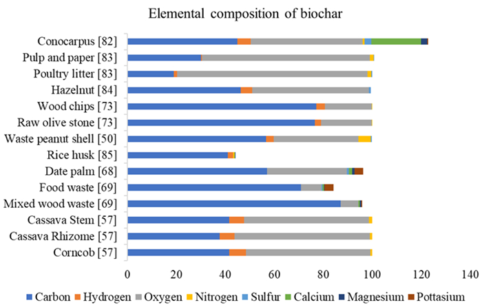
Wijitkosum S, Jiwnok P (2019) Elemental composition of biochar obtained from agricultural waste for soil amendment and carbon sequestration. App Sci 9: 3980. https://doi:10.3390/app9193980 doi: 10.3390/app9193980
![]() |
[58] |
Liu W, Li K, Xu S (2022) Utilizing bamboo biochar in cement mortar as a bio-modifier to improve the compressive strength and crack-resistance fracture ability. Constr Build Mater 327: 126917. https://doi:10.1016/j.conbuildmat.2022.126917 doi: 10.1016/j.conbuildmat.2022.126917
![]() |
[59] |
Graber ER, Tsechansky L, Gerstl Z, et al. (2012) High surface area biochar negatively impacts herbicide efficacy. Plant Soil 353: 95–106. https://doi:10.1007/s11104-011-1012-7 doi: 10.1007/s11104-011-1012-7
![]() |
[60] |
Peterson SC, Jackson MA, Kim S, et al (2012) Increasing biochar surface area: Optimization of ball milling parameters. Powder Technol 228: 115–120. https://doi:10.1016/J.POWTEC.2012.05.005 doi: 10.1016/J.POWTEC.2012.05.005
![]() |
[61] |
Xu D, Cao J, Li Y, et al. (2019) Effect of pyrolysis temperature on characteristics of biochars derived from different feedstocks: A case study on ammonium adsorption capacity. Waste Manage 87: 652–660. https://doi:10.1016/j.wasman.2019.02.049 doi: 10.1016/j.wasman.2019.02.049
![]() |
[62] |
Wani I, Sharma A, Kushvaha V, et al. (2020). Effect of pH, volatile content, and pyrolysis conditions on surface area and O/C and H/C ratios of biochar: towards understanding performance of biochar using simplified approach. J Hazard Toxic Radioact Waste 24: 04020048. https://doi:10.1061/(asce)hz.2153-5515.0000545 doi: 10.1061/(asce)hz.2153-5515.0000545
![]() |
[63] |
Gao Y, Zhang Y, Li A, et al. (2018) Facile synthesis of high-surface area mesoporous biochar for energy storage via in-situ template strategy. Mater Lett 230: 183–186. https://doi:10.1016/j.matlet.2018.07.106 doi: 10.1016/j.matlet.2018.07.106
![]() |
[64] |
Chia CH, Gong B, Joseph SD, et al. (2012) Imaging of mineral-enriched biochar by FTIR, Raman and SEM–EDX. Vib Spectrosc 62: 248–257. https://doi:10.1016/J.VIBSPEC.2012.06.006 doi: 10.1016/J.VIBSPEC.2012.06.006
![]() |
[65] | Danish A, Mosaberpanah MA, Salim MU, et al. (2021) Reusing biochar as a filler or cement replacement material in cementitious composites: A review. Constr Build Mater 300: 124295. https://doi.10.1016/j.conbuildmat.2021.124295 |
[66] | Khiari B, Ghouma I, Ferjani AI, et al. (2020) Kenaf stems: Thermal characterization and conversion for biofuel and biochar production. Fuel 262: 116654. https://doi.10.1016/j.fuel.2019.116654 |
[67] |
Gupta S, Krishnan P, Kashani A, et al. (2020) Application of biochar from coconut and wood waste to reduce shrinkage and improve physical properties of silica fume-cement mortar. Constr Build Mater 262: 120688. https://doi:10.1016/j.conbuildmat.2020.120688 doi: 10.1016/j.conbuildmat.2020.120688
![]() |
[68] |
Elnour AY, Alghyamah AA, Shaikh HM, et al. (2019) Effect of pyrolysis temperature on biochar microstructural evolution, physicochemical characteristics, and its influence on biochar/polypropylene composites. Appl Sci 9: 1149. https://doi.org/10.3390/app9061149. doi: 10.3390/app9061149
![]() |
[69] |
Gupta S, Kua HW, Koh HJ (2018) Application of biochar from food and wood waste as green admixture for cement mortar. Sci Total Environ 619: 419–435. https://doi:10.1016/j.scitotenv.2017.11.044 doi: 10.1016/j.scitotenv.2017.11.044
![]() |
[70] |
Ahmad MR, Chen B, Duan H (2020) Improvement effect of pyrolyzed agro-food biochar on the properties of magnesium phosphate cement. Sci Total Environ 718: 137422. https://doi:10.1016/j.scitotenv.2020.137422 doi: 10.1016/j.scitotenv.2020.137422
![]() |
[71] |
Zeidabadi ZA, Bakhtiari S, Abbaslou H, et al. (2018) Synthesis, characterization and evaluation of biochar from agricultural waste biomass for use in building materials. Constr Build Mater 181: 301–308. https://doi:10.1016/j.conbuildmat.2018.05.271 doi: 10.1016/j.conbuildmat.2018.05.271
![]() |
[72] |
Maljaee H, Madadi R, Paiva H, et al. (2021) Sustainable lightweight mortar using biochar as sand replacement. Eur J Environ Civ Eng 26: 8263–8279. https://doi:10.1080/19648189.2021.2021998 doi: 10.1080/19648189.2021.2021998
![]() |
[73] |
Maljaee H, Paiva H, Madadi R, et al. (2021) Effect of cement partial substitution by waste-based biochar in mortars properties. Constr Build Mater 301: 124074. https://doi:10.1016/j.conbuildmat.2021.124074 doi: 10.1016/j.conbuildmat.2021.124074
![]() |
[74] |
Ahmed MB, Zhou JL, Ngo HH, et al. (2016) Insight into biochar properties and its cost analysis. Biomass Bioenerg 84: 76–86. https://doi:10.1016/j.biombioe.2015.11.002 doi: 10.1016/j.biombioe.2015.11.002
![]() |
[75] |
Li C, Hayashi JI, Sun Y, et al. (2021) Impact of heating rates on the evolution of function groups of the biochar from lignin pyrolysis. J Anal Appl Pyrolysis 155: 105031. https://doi:10.1016/J.JAAP.2021.105031 doi: 10.1016/J.JAAP.2021.105031
![]() |
[76] |
Claoston N, Samsuri AW, Ahmad Husni MH, et al. (2014) Effects of pyrolysis temperature on the physicochemical properties of empty fruit bunch and rice husk biochars. Waste Manag Res 32: 331–339. https://doi:10.1177/0734242X14525822 doi: 10.1177/0734242X14525822
![]() |
[77] |
Zhang Y, Ma Z, Zhang Q, et al. (2017) Comparison of the physicochemical characteristics of bio-char pyrolyzed from moso bamboo and rice husk with different pyrolysis temperatures. BioResources 12: 4652–4669. https://doi:10.15376/BIORES.12.3.4652-4669 doi: 10.15376/BIORES.12.3.4652-4669
![]() |
[78] |
Crombie K, Mašek O, Sohi SP, et al. (2013) The effect of pyrolysis conditions on biochar stability as determined by three methods. Gcb Bioenergy 5: 122–131. https://doi:10.1111/GCBB.12030 doi: 10.1111/GCBB.12030
![]() |
[79] |
He M, Xu Z, Sun Y, et al. (2021) Critical impacts of pyrolysis conditions and activation methods on application-oriented production of wood waste-derived biochar. Bioresource Technol 341: 125811. https://doi:10.1016/J.biortech.2021.125811 doi: 10.1016/J.biortech.2021.125811
![]() |
[80] |
Ye L, Zhang J, Zhao J, et al. (2015) Properties of biochar obtained from pyrolysis of bamboo shoot shell. J Anal Appl Pyrolysis 114: 172–178. https://doi: 10.1016/j.jaap.2015.05.016. doi: 10.1016/j.jaap.2015.05.016
![]() |
[81] |
Liu Z, Fei B, Jiang Z (2014) Combustion characteristics of bamboo-biochars. Bioresource Technol 167: 94–99. https://doi:10.1016/j.biortech.2014.05.023 doi: 10.1016/j.biortech.2014.05.023
![]() |
[82] |
Al-Wabel MI, Al-Omran A, El-Naggar AH, et al. (2013) Pyrolysis temperature induced changes in characteristics and chemical composition of biochar produced from conocarpus wastes. Bioresource Technol 131: 374–379. https://doi.org/10.1016/j.biortech.2012.12.165 doi: 10.1016/j.biortech.2012.12.165
![]() |
[83] |
Akhtar A, Sarmah AK (2018) Novel biochar-concrete composites: Manufacturing, characterization and evaluation of the mechanical properties. Sci Total Environ 616: 408–416. https://doi:10.1016/j.scitotenv.2017.10.319 doi: 10.1016/j.scitotenv.2017.10.319
![]() |
[84] |
Zhao C, Liu X, Chen A, et al. (2020) Characteristics evaluation of bio-char produced by pyrolysis from waste hazelnut shell at various temperatures. Energ Source Part A 1–11. https://doi.org/10.1080/15567036.2020.1754530 doi: 10.1080/15567036.2020.1754530
![]() |
[85] |
Gupta S, Kua HW (2020) Application of rice husk biochar as filler in cenosphere modified mortar: Preparation, characterization and performance under elevated temperature. Constr Build Mater 253: 119083. https://doi:10.1016/j.conbuildmat.2020.119083 doi: 10.1016/j.conbuildmat.2020.119083
![]() |
[86] | ASTM International (2003) Standard specification for coal fly ash and raw or calcined natural pozzolan for use in concrete. ASTM 619-03. |
[87] |
Zeidabadi ZA, Bakhtiari S, Abbaslou H, et al. (2018) Synthesis, characterization and evaluation of biochar from agricultural waste biomass for use in building materials. Constr Build Mater 181: 301–308. https://doi:10.1016/j.conbuildmat.2018.05.271 doi: 10.1016/j.conbuildmat.2018.05.271
![]() |
[88] | ASTM International (2019) Standard specification for coal fly ash and raw or calcined natural pozzolan for use in concrete. ASTM 619-19. |
[89] |
Jeon J, Kim HI, Park JH, et al. (2021) Evaluation of thermal properties and acetaldehyde adsorption performance of sustainable composites using waste wood and biochar. Environ Res 196: 110910. https://doi:10.1016/j.envres.2021.110910 doi: 10.1016/j.envres.2021.110910
![]() |
[90] |
Ngo T, Khudur LS, Hakeem IG, et al. (2022) Wood biochar enhances the valorisation of the anaerobic digestion of chicken manure. Clean Technol Environ Policy 4: 420–439. https://doi:10.3390/cleantechnol4020026 doi: 10.3390/cleantechnol4020026
![]() |
[91] |
Dixit A, Gupta S, Dai Pang S, et al. (2019) Waste valorisation using biochar for cement replacement and internal curing in ultra-high performance concrete. J Clean Prod 238: 117876. https://doi.org/10.1016/j.jclepro.2019.117876 doi: 10.1016/j.jclepro.2019.117876
![]() |
[92] |
Rehrah D, Bansode RR, Hassan O, et al. (2016) Physico-chemical characterization of biochars from solid municipal waste for use in soil amendment. J Anal Appl Pyrolysis 118: 42–53. https://doi:10.1016/J.JAAP.2015.12.022. doi: 10.1016/J.JAAP.2015.12.022
![]() |
[93] |
Silber A, Levkovitch I, Graber ER (2010) pH-dependent mineral release and surface properties of cornstraw biochar: agronomic implications. Environ Sci Technol 44: 9318–9323. https://doi.org/10.1021/es101283d. doi: 10.1021/es101283d
![]() |
[94] |
Gonzalez J, Sargent P, Ennis C (2021) Sewage treatment sludge biochar activated blast furnace slag as a low carbon binder for soft soil stabilisation. J Clean Prod 311: 127553. https://doi:10.1016/j.jclepro.2021.127553. doi: 10.1016/j.jclepro.2021.127553
![]() |
[95] |
Yuan JH, Xu RK (2011) The amelioration effects of low temperature biochar generated from nine crop residues on an acidic Ultisol. Soil Use Manag 27: 110–115. https://doi:10.1111/j.1475-2743.2010.00317.x doi: 10.1111/j.1475-2743.2010.00317.x
![]() |
[96] |
Cosentino I, Restuccia L, Ferro GA, et al. (2019) Type of materials, pyrolysis conditions, carbon content and size dimensions: The parameters that influence the mechanical properties of biochar cement-based composites. Theor Appl Fract Mech 103: 102261. https://doi:10.1016/j.tafmec.2019.102261. doi: 10.1016/j.tafmec.2019.102261
![]() |
[97] |
Malhotra HL (1956) The effect of temperature on the compressive strength of concrete. Mag Concr Res 8: 85–94. https://doi.org/10.1680/macr.1956.8.23.85 doi: 10.1680/macr.1956.8.23.85
![]() |
[98] |
Khoury GA (1992) Compressive strength of concrete at high temperatures: a reassessment. Mag Concr Res 44: 291–309. https://doi:10.1680/MACR.1992.44.161.291 doi: 10.1680/MACR.1992.44.161.291
![]() |
[99] |
Jang JG, Lee HK (2016) Microstructural densification and CO2 uptake promoted by the carbonation curing of belite-rich Portland cement. Cem Concr Res 82: 50–57. https://doi:10.1016/j.cemconres.2016.01.001 doi: 10.1016/j.cemconres.2016.01.001
![]() |
[100] |
Han T (2020) Application of peanut biochar as admixture in cement mortar. IOP Conf Ser-Earth Environ Sci 531: 012061. https://doi:10.1088/1755-1315/531/1/012061 doi: 10.1088/1755-1315/531/1/012061
![]() |
[101] |
Gupta S, Kua HW (2018) Effect of water entrainment by pre-soaked biochar particles on strength and permeability of cement mortar. Constr Build Mater 159: 107–125. https://doi:10.1016/j.conbuildmat.2017.10.095 doi: 10.1016/j.conbuildmat.2017.10.095
![]() |
[102] |
Sirico A, Bernardi P, Belletti B, et al. (2020) Mechanical characterization of cement-based materials containing biochar from gasification. Constr Build Mater 246: 118490. https://doi:10.1016/j.conbuildmat.2020.118490 doi: 10.1016/j.conbuildmat.2020.118490
![]() |
[103] |
Wang L, Chen L, Tsang DC, et al. (2020) Biochar as green additives in cement-based composites with carbon dioxide curing. J Clean Prod 258: 120678. https://doi:10.1016/j.jclepro.2020.120678 doi: 10.1016/j.jclepro.2020.120678
![]() |
[104] |
Birchall JD, Howard AJ, Kendall K (1981) Flexural strength and porosity of cements. Nature 289: 388–390. https://doi:10.1038/289388a0 doi: 10.1038/289388a0
![]() |
[105] |
Bowlby LK, Saha GC, Afzal MT (2018) Flexural strength behavior in pultruded GFRP composites reinforced with high specific-surface-area biochar particles synthesized via microwave pyrolysis. Composites Part A-Appl S 110: 190–196. https://doi:10.1016/j.compositesa.2018.05.003 doi: 10.1016/j.compositesa.2018.05.003
![]() |
[106] |
Cosentino I, Restuccia L, Ferro GA (2019) Type of materials, pyrolysis conditions, carbon content and size dimensions: The parameters that influence the mechanical properties of biochar cement-based composites. Theor Appl Fract Mech 103: 102261. https://doi:10.1016/j.tafmec.2019.102261 doi: 10.1016/j.tafmec.2019.102261
![]() |
[107] |
Das O, Kim NK, Kalamkarov AL, et al. (2017). Biochar to the rescue: Balancing the fire performance and mechanical properties of polypropylene composites. Polym Degrad Stab 144: 485–496. https://doi: 10.1016/j.polymdegradstab.2017.09.006 doi: 10.1016/j.polymdegradstab.2017.09.006
![]() |
[108] |
Ahmad S, Tulliani JM, Ferro GA, et al. (2015) Crack path and fracture surface modifications in cement composites. Frat ed Integrita Strutt 9: 34. https://doi:10.3221/igf-esis.34.58 doi: 10.3221/igf-esis.34.58
![]() |
[109] |
Gupta S, Kua HW, Low CY (2018) Use of biochar as carbon sequestering additive in cement mortar. Cem Concr Compos 87: 110–129. https://doi:10.1016/j.cemconcomp.2017.12.009 doi: 10.1016/j.cemconcomp.2017.12.009
![]() |
[110] |
Chen B, Li C, Chen L (2009) Experimental study of mechanical properties of normal-strength concrete exposed to high temperatures at an early age. Fire Saf J 44: 997–1002. https://doi:10.1016/j.firesaf.2009.06.007 doi: 10.1016/j.firesaf.2009.06.007
![]() |
[111] |
Gupta S, Kua HW, Dai Pang S (2020) Effect of biochar on mechanical and permeability properties of concrete exposed to elevated temperature. Constr Build Mater 234: 117338. https://doi:10.1016/j.conbuildmat.2019.117338 doi: 10.1016/j.conbuildmat.2019.117338
![]() |
[112] |
Chen X, Wu S, Zhou J (2013) Influence of porosity on compressive and tensile strength of cement mortar. Constr Build Mater 40: 869–874. https://doi:10.1016/J.CONBUILDMAT.2012.11.072 doi: 10.1016/J.CONBUILDMAT.2012.11.072
![]() |
[113] |
Hossain MM, Karim MR, Hasan M, et al. (2016) Durability of mortar and concrete made up of pozzolans as a partial replacement of cement: A review. Constr Build Mater 116: 128–140. https://doi:10.1016/j.conbuildmat.2016.04.147 doi: 10.1016/j.conbuildmat.2016.04.147
![]() |
[114] |
Gupta S, Muthukrishnan S, Kua HW (2021) Comparing influence of inert biochar and silica rich biochar on cement mortar–Hydration kinetics and durability under chloride and sulfate environment. Constr Build Mater 268: 121142. https://doi:10.1016/j.conbuildmat.2020.121142 doi: 10.1016/j.conbuildmat.2020.121142
![]() |
[115] |
Zanotto F, Sirico A, Merchiori S, et al. (2022) Durability of reinforced concrete containing biochar and recycled polymers. Key Eng Mater 919: 188–196. https://doi.org/10.4028/p-mwn300 doi: 10.4028/p-mwn300
![]() |
[116] |
Cuthbertson D, Berardi U, Briens C, et al. (2019) Biochar from residual biomass as a concrete filler for improved thermal and acoustic properties. Biomass Bioenerg 120: 77–83. https://doi:10.1016/j.biombioe.2018.11.007 doi: 10.1016/j.biombioe.2018.11.007
![]() |
[117] |
Wang L, Chen L, Tsang DC, et al. (2019) The roles of biochar as green admixture for sediment-based construction products. Cem Concr Compos 104: 103348. https://doi:10.1016/j.cemconcomp.2019.103348 doi: 10.1016/j.cemconcomp.2019.103348
![]() |
[118] |
Legan M, Gotvajn AŽ, Zupan K (2022) Potential of biochar use in building materials. J Environ Manage 309: 114704. https://doi:10.1016/j.jenvman.2022.114704 doi: 10.1016/j.jenvman.2022.114704
![]() |
[119] |
Berardi U, Naldi M (2017) The impact of the temperature dependent thermal conductivity of insulating materials on the effective building envelope performance. Energ Buildings 144: 262–275. https://doi:10.1016/j.enbuild.2017.03.052 doi: 10.1016/j.enbuild.2017.03.052
![]() |
[120] |
Tan K, Qin Y, Wang J (2022) Evaluation of the properties and carbon sequestration potential of biochar-modified pervious concrete. Constr Build Mater 314: 125648. https://doi:10.1016/j.conbuildmat.2021.125648 doi: 10.1016/j.conbuildmat.2021.125648
![]() |
[121] |
Gupta S, Kua HW (2017) Factors determining the potential of biochar as a carbon capturing and sequestering construction material: critical review. J Mater Civ Eng 29: 04017086. https://doi:10.1061/(asce)mt.1943-5533.0001924 doi: 10.1061/(asce)mt.1943-5533.0001924
![]() |
[122] |
Maljaee H, Madadi R, Paiva H, et al. (2021) Sustainable lightweight mortar using biochar as sand replacement. Eur J Environ Civ Eng 26: 8263–8279. https://doi.org/10.1080/19648189.2021.2021998 doi: 10.1080/19648189.2021.2021998
![]() |
[123] |
Gupta S, Kua HW (2020) Combination of biochar and silica fume as partial cement replacement in mortar: Performance evaluation under normal and elevated temperature. Waste Biomass Valori 11: 2807–2824. https://doi:10.1007/s12649-018-00573-x. doi: 10.1007/s12649-018-00573-x
![]() |
[124] |
Restuccia L, Ferro GA (2016) Promising low cost carbon-based materials to improve strength and toughness in cement composites. Constr Build Mater 126: 1034–1043. https://doi:10.1016/j.conbuildmat.2016.09.101 doi: 10.1016/j.conbuildmat.2016.09.101
![]() |
[125] |
Mrad R, Chehab, G (2019). Mechanical and microstructure properties of biochar-based mortar: An internal curing agent for PCC. Sustainability 11: 2491. https://doi.org/10.3390/su11092491 doi: 10.3390/su11092491
![]() |
[126] |
Maljaee H, Madadi R, Paiva H, et al. (2021) Incorporation of biochar in cementitious materials: A roadmap of biochar selection. Constr Build Mater 283: 122757. https://doi.org/10.1016/j.conbuildmat.2021.122757 doi: 10.1016/j.conbuildmat.2021.122757
![]() |
[127] |
Restuccia, L, Ferro GA, Suarez-Riera D, et al. (2020). Mechanical characterization of different biochar-based cement composites. Procedia Struct Integr 25: 226–233. https://doi.org/10.1016/j.prostr.2020.04.027 doi: 10.1016/j.prostr.2020.04.027
![]() |
1. | Hassan K. Ahmad, Michael R. Milne, Quinlan D. Buchlak, Nalan Ektas, Georgina Sanderson, Hadi Chamtie, Sajith Karunasena, Jason Chiang, Xavier Holt, Cyril H. M. Tang, Jarrel C. Y. Seah, Georgina Bottrell, Nazanin Esmaili, Peter Brotchie, Catherine Jones, Machine Learning Augmented Interpretation of Chest X-rays: A Systematic Review, 2023, 13, 2075-4418, 743, 10.3390/diagnostics13040743 | |
2. | F. M. Javed Mehedi Shamrat, Sami Azam, Asif Karim, Rakibul Islam, Zarrin Tasnim, Pronab Ghosh, Friso De Boer, LungNet22: A Fine-Tuned Model for Multiclass Classification and Prediction of Lung Disease Using X-ray Images, 2022, 12, 2075-4426, 680, 10.3390/jpm12050680 | |
3. | Mavra Mehmood, Nasser Alshammari, Saad Awadh Alanazi, Asma Basharat, Fahad Ahmad, Muhammad Sajjad, Kashaf Junaid, Improved colorization and classification of intracranial tumor expanse in MRI images via hybrid scheme of Pix2Pix-cGANs and NASNet-large, 2022, 34, 13191578, 4358, 10.1016/j.jksuci.2022.05.015 | |
4. | Medha Jha, Yasha Hasija, 2023, Artificial Intelligence In Field of Medical Imaging Informatics, 979-8-3503-9926-4, 661, 10.1109/ICACITE57410.2023.10182498 | |
5. | Mélanie Champendal, Henning Müller, John O. Prior, Cláudia Sá dos Reis, A scoping review of interpretability and explainability concerning artificial intelligence methods in medical imaging, 2023, 169, 0720048X, 111159, 10.1016/j.ejrad.2023.111159 | |
6. | Afshin Shoeibi, Marjane Khodatars, Mahboobeh Jafari, Navid Ghassemi, Delaram Sadeghi, Parisa Moridian, Ali Khadem, Roohallah Alizadehsani, Sadiq Hussain, Assef Zare, Zahra Alizadeh Sani, Fahime Khozeimeh, Saeid Nahavandi, U. Rajendra Acharya, Juan M. Gorriz, Automated detection and forecasting of COVID-19 using deep learning techniques: A review, 2024, 577, 09252312, 127317, 10.1016/j.neucom.2024.127317 | |
7. | Samuel Enobong Sunday, Lie Liu, Huang Fei, Yongfei Ju, Hong Ki An, 2024, A Smart Hybrid Model for Fruit Quality Grading: Merging Canny Edge Detection and K-means Clustering Algorithm, 979-8-3503-5289-4, 320, 10.1109/ICCD62811.2024.10843620 | |
8. | Mohamed Tounsi, Erahid Aram, Ahmad Taher Azar, Ahmed Al-Khayyat, Ibraheem Kasim Ibraheem, A Comprehensive Review on Biomedical Image Classification using Deep Learning Models, 2025, 15, 1792-8036, 19538, 10.48084/etasr.8728 | |
9. | Burcu Oltu, Selda Güney, Seniha Esen Yuksel, Berna Dengiz, Automated classification of chest X-rays: a deep learning approach with attention mechanisms, 2025, 25, 1471-2342, 10.1186/s12880-025-01604-5 |
Disease | Train set | Test set | Val set |
Nodule | 1890 | 550 | 270 |
Atelectasis | 2940 | 840 | 420 |
Normal | 2200 | 612 | 310 |
Infection | 2360 | 670 | 320 |
layer | Output size | Kernel size | channel |
Input(224 × 224 × 3) | |||
A | 112 × 112 | 3, 5, 7 | 45 |
AdaptiveAvgPool (2 × 2, stride = 1) | |||
B × 4 | 56 × 56 | 3 | 45 |
A | 28 × 28 | 3, 5, 7 | 135 |
B × 4 | 28 × 28 | 3 | 135 |
A | 14 × 14 | 3, 5, 7 | 405 |
B × 6 | 14 × 14 | 3 | 405 |
A | 7 × 7 | 3, 5, 7 | 1215 |
B × 6 | 7 × 7 | 3 | 1215 |
AvgPool (kernel_size = 7, stride = 1) | |||
Linear (output = 4) |
Model | Disease | Precision | Recall | F1-score | AUC |
MARnet | Nodule | 69.85 ±0.1 | 58.55 ±0.1 | 59.46 ±0.1 | 0.90 |
Atelectasis | 75.88 ±0.1 | 85.00 ±0.1 | 76.49 ±0.1 | 0.93 | |
Normal | 98.50 ±0.1 | 86.90 ±0.9 | 70.50 ±0.4 | 0.99 | |
Infection | 91.03 ±0.1 | 98.51 ±0.1 | 75.04 ±0.1 | 1.00 | |
MRnet | Nodule | 63.21 ±0.1 | 24.44 ±0.1 | 35.97 ±0.1 | 0.85 |
Atelectasis | 64.69 ±0.1 | 91.12±0.2 | 75.59 ±0.2 | 0.89 | |
Normal | 98.79 ± 0.2 | 80.87 ±0.1 | 88.85 ±0.1 | 0.67 | |
Infection | 85.91 ±0.1 | 98.72 ±0.1 | 91.38±0.1 | 0.95 | |
ARnet | Nodule | 55.10 ± 1.4 | 55.60 ± 1.2 | 55.41 ± 1.4 | 0.86 |
Atelectasis | 72.20 ±0.1 | 71.78 ±0.2 | 72.04 ±0.1 | 0.90 | |
Normal | 96.68 ±0.1 | 75.46 ±0.1 | 84.83 ±0.1 | 0.90 | |
Infection | 81.57 ±0.1 | 97.92 ±0.1 | 89.04 ±0.2 | 0.98 | |
FAnet | Nodule | 64.84 ± 0.2 | 55.02 ±0.2 | 59.01 ±0.1 | 0.88 |
Atelectasis | 73.13 ±0.1 | 80.12 ±0.1 | 76.46 ±0.1 | 0.90 | |
Normal | 98.30 ±0.1 | 86.85 ±0.2 | 92.12 ±0.2 | 0.94 | |
Infection | 89.75 ±0.1 | 98.41 ± 1.0 | 92.82 ±0.3 | 0.99 |
Model | Disease | Precision | Recall | F1-score | AUC |
MARnet | Nodule | 69.85 ±0.1 | 58.55 ±0.1 | 59.46 ±0.1 | 0.90 |
Atelectasis | 75.88 ±0.1 | 85.00 ±0.1 | 76.49 ±0.1 | 0.93 | |
Normal | 98.50 ±0.1 | 86.90 ±0.9 | 70.50 ±0.4 | 0.99 | |
Infection | 91.03 ±0.1 | 98.51 ±0.1 | 75.04 ±0.1 | 1.00 | |
AlexNet | Nodule | 46.31 ±0.1 | 12.54 ±0.1 | 14.79 ±0.1 | 0.69 |
Atelectasis | 61.49 ±0.1 | 89.52 ±0.1 | 65.39 ±0.1 | 0.87 ±0.01 | |
Normal | 93.79 ±0.1 | 66.67 ±0.1 | 50.65 ±0.1 | 0.89 | |
Infection | 74.91 ±0.1 | 96.72 ±0.1 | 61.98 ±0.1 | 0.97 | |
VGG16 | Nodule | 59.50 ±2.6 | 34.00 ±2.2 | 37.20 ± 1.4 | 0.87 |
Atelectasis | 67.20 ±0.1 | 90.00 ±0.1 | 70.49 ±0.1 | 0.91 ±0.01 | |
Normal | 97.78 ±0.1 | 72.06 ±0.1 | 58.23 ±0.1 | 0.98 | |
Infection | 83.51 ±0.1 | 95.97 ±0.1 | 70.14 ±0.1 | 0.98 | |
InceptionV2 | Nodule | 58.94 ±0.1 | 42.55 ±0.1 | 42.01 ±0.1 | 0.88 ±0.01 |
Atelectasis | 69.03 ±0.1 | 81.19±0.1 | 67.86 ±0.1 | 0.91 ± 0.01 | |
Normal | 95.50 ± 1.0 | 73.00 ± 1.2 | 57.80 ±0.7 | 0.97 | |
Infection | 80.25 ± 0.2 | 97.00 ± 1.0 | 66.80 ±0.4 | 0.98 | |
ResNet101 | Nodule | 55.00 ± 1.2 | 12.00 ±0.7 | 16.20 ±0.6 | 0.87 ±0.01 |
Atelectasis | 63.06 ±0.1 | 95.71 ±0.1 | 69.91 ±0.1 | 0.92 | |
Normal | 97.20 ±0.1 | 73.50 ±0.1 | 56.50 ±0.3 | 0.97 | |
Infection | 80.91 ±0.1 | 98.06 ±0.1 | 65.50 ±0.1 | 0.99 | |
CliqueNet | Nodule | 57.20 ± 1.5 | 31.50± 1.6 | 33.00 ± 1.5 | 0.85 |
Atelectasis | 66.67 ±0.1 | 86.19±0.1 | 67.14 ±0.1 | 0.91 ±0.01 | |
Normal | 94.79 ±0.1 | 68.30 ±0.1 | 54.46 ±0.1 | 0.84 | |
Infection | 77.73 ±0.1 | 96.87 ±0.1 | 65.00 ±0.1 | 0.96 |
Disease | CheXNet | GraphXNet | TieNet | AM_DenseNet | MARnet |
Nodule | 0.78 | 0.71 | 0.69 | 0.81 | 0.90 |
Atelectasis | 0.81 | 0.72 | 0.73 | 0.83 | 0.93 |
Normal | - | - | 0.70 | - | 0.99 |
Infection | 0.79 | 0.76 | 0.71 | 0.80 | 1.00 |