In our paper, a delayed diffusive phytoplankton-zooplankton-fish model with a refuge and Crowley-Martin and Holling II functional responses is established. First, for the model without delay and diffusion, we not only analyze the existence and stability of equilibria, but also discuss the occurrence of Hopf bifurcation by choosing the refuge proportion of phytoplankton as the bifurcation parameter. Then, for the model with delay, we set some sufficient conditions to demonstrate the existence of Hopf bifurcation caused by delay; we also discuss the direction of Hopf bifurcation and the stability of the bifurcation of the periodic solution by using the center manifold and normal form theories. Next, for a reaction-diffusion model with delay, we show the existence and properties of Hopf bifurcation. Finally, we use Matlab software for numerical simulation to prove the previous theoretical results.
Citation: Ting Gao, Xinyou Meng. Stability and Hopf bifurcation of a delayed diffusive phytoplankton-zooplankton-fish model with refuge and two functional responses[J]. AIMS Mathematics, 2023, 8(4): 8867-8901. doi: 10.3934/math.2023445
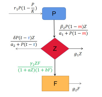
In our paper, a delayed diffusive phytoplankton-zooplankton-fish model with a refuge and Crowley-Martin and Holling II functional responses is established. First, for the model without delay and diffusion, we not only analyze the existence and stability of equilibria, but also discuss the occurrence of Hopf bifurcation by choosing the refuge proportion of phytoplankton as the bifurcation parameter. Then, for the model with delay, we set some sufficient conditions to demonstrate the existence of Hopf bifurcation caused by delay; we also discuss the direction of Hopf bifurcation and the stability of the bifurcation of the periodic solution by using the center manifold and normal form theories. Next, for a reaction-diffusion model with delay, we show the existence and properties of Hopf bifurcation. Finally, we use Matlab software for numerical simulation to prove the previous theoretical results.

| [1] | E. P. Odum, Fundamentals of ecology, Philadelphia: W. B. Saunders Company, 1953. |
| [2] |
J. J. Cole, S. R. Carpenter, M. L. Pace, Differential support of lake food web by three types of terrestrial organic carbon, Ecol. Lett., 9 (2006), 558–568. https://doi.org/10.1111/j.1461-0248.2006.00898.x doi: 10.1111/j.1461-0248.2006.00898.x

|
| [3] |
W. Edmondson, Reproductive rate of planktonic rotifers as related to food and temperature in nature, Ecol. Monogr., 35 (1965), 61–111. https://doi.org/10.2307/1942218 doi: 10.2307/1942218
|
| [4] |
X. W. Yu, S. L. Yuan, T. H. Zhang, Survival and ergodicity of a stochastic phytoplankton-zooplankton model with toxin-producing phytoplankton in an impulsive polluted environment, Appl. Math. Comput., 347 (2019), 249–264. https://doi.org/10.1016/j.amc.2018.11.005 doi: 10.1016/j.amc.2018.11.005
|
| [5] |
R. H. Fleming, The control of diatom populations by grazing, ICES J. Mar. Sci., 14 (1939), 210–227. https://doi.org/10.1093/icesjms/14.2.210 doi: 10.1093/icesjms/14.2.210
|
| [6] |
E. Beltrami, T. O. Carroll, Modeling the role of viral disease in recurrent phytoplankton blooms, J. Math. Biol., 32 (1994), 857–863. https://doi.org/10.1007/BF00168802 doi: 10.1007/BF00168802
|
| [7] |
J. Norberg, D. DeAngelis, Temperature effects on stocks and stability of a phytoplankton-zooplankton model and the dependence on light and nutrients, Ecol. Modell., 95 (1997), 75–86. https://doi.org/10.1016/S0304-3800(96)00033-6 doi: 10.1016/S0304-3800(96)00033-6
|
| [8] |
B. Mukhopadhyay, R. Bhattacharyya, Modelling phytoplankton allelopathy in a nutrient-plankton model with spatial heterogeneity, Ecol. Modell., 198 (2006), 163–173. https://doi.org/10.1016/j.ecolmodel.2006.04.005 doi: 10.1016/j.ecolmodel.2006.04.005
|
| [9] |
S. Pal, S. Chatterjee, J. Chattopadhyay, Role of toxin and nutrient for the occurrence and termination of plankton bloom-results drawn from field observations and a mathematical model, Biosystems, 90 (2007), 87–100. doi: 10.1016/j.biosystems.2006.07.003 doi: 10.1016/j.biosystems.2006.07.003
|
| [10] |
T. Saha, M. Bandyopadhyay, Dynamical analysis of toxin producing phytoplankton-zooplankton interactions, Nonlinear Anal. Real World Appl., 10 (2009), 314–332. doi:10.3934/mbe.2017032 doi: 10.3934/mbe.2017032
|
| [11] |
J. Chattopadhayay, R. R. Sarkar, S. Mandal, Toxin-producing plankton may act as a biological control for planktonic blooms-field study and mathematical modelling, J. Theor. Biol., 215 (2002), 333–344. doi:10.1006/jtbi.2001.2510 doi: 10.1006/jtbi.2001.2510
|
| [12] |
J. B. Collings, Bifurcation and stability analysis of a temperature-dependent mite predator prey interaction model incorporating a prey refuge, Bull. Math. Biol., 57 (1995), 63–76. https://doi.org/10.1016/0092-8240(94)00024-7 doi: 10.1016/0092-8240(94)00024-7
|
| [13] |
G. O. Eduardo, R. J. Rodrigo, Dynamic consequences of prey refuges in a simple model system: more prey, fewer predators and enhanced stability, Ecol. Modell., 166 (2003), 135–146. https://doi.org/10.1016/S0304-3800(03)00131-5 doi: 10.1016/S0304-3800(03)00131-5
|
| [14] |
L. J. Chen, F. D. Chen, L. J. Chen, Qualitative analysis of a predator-rey model with Holling type II functional response incorporating a constant prey refuge, Nonlinear Anal. Real World Appl., 11 (2008), 246–252. https://doi.org/10.1016/j.nonrwa.2008.10.056 doi: 10.1016/j.nonrwa.2008.10.056
|
| [15] |
D. E. Schindler, M. D. Scheuerell, Habitat coupling in lake ecosystems, Oikos, 98 (2002), 177–189. https://doi.org/10.1034/j.1600-0706.2002.980201.x doi: 10.1034/j.1600-0706.2002.980201.x
|
| [16] |
P. J. Wiles, L. A. V. Duren, C. Hase, Stratification and mixing in the Limfjorden in relation to mussel culture, J. Mar. Syst., 60 (2006), 129–143. https://doi.org/10.1016/j.jmarsys.2005.09.009 doi: 10.1016/j.jmarsys.2005.09.009
|
| [17] |
M. M. Mullin, J. F. Frederick, Ingestion by planktonic grazers as a function of concentration of food, Limnol. Oceanogr., 20 (1975), 259–262. https://doi.org/10.4319/lo.1975.20.2.0259 doi: 10.4319/lo.1975.20.2.0259
|
| [18] |
J. Li, Y. Z. Song, H. Wan, H. P. Zhu, Dynamical analysis of a toxin-producing phytoplankton-zooplankton model with refuge, Math. Biosci. Eng., 14 (2017), 529–557. https://doi.org/10.3934/mbe.2017032 doi: 10.3934/mbe.2017032
|
| [19] |
J. L. Zhao, Y. Yan, L. Z. Huang, R. Yang, Delay driven Hopf bifurcation and chaos in a diffusive toxin producing phytoplankton-zooplankton model, Math. Methods Appl. Sci., 42 (2019), 3831–3847. https://doi.org/10.1002/mma.5615 doi: 10.1002/mma.5615
|
| [20] |
G. D. Liu, X. Z. Meng, S. Y. Liu, Dynamics for a tritrophic impulsive periodic plankton-fish system with diffusion in lakes, Math. Methods Appl. Sci., 44 (2020), 3260–3279. https://doi.org/10.1002/mma.6938 doi: 10.1002/mma.6938
|
| [21] |
X. Y. Meng, L. Xiao, Stability and bifurcation for a delayed diffusive two-zooplankton one-phytoplankton model with two different functions, Complexity, 2021 (2021), 5560157. https://doi.org/10.1155/2021/5560157 doi: 10.1155/2021/5560157
|
| [22] |
M. L. Rosenzweig, Paradox of enrichment: destabilization of exploitation systems in ecological time, Sci. Rep., 171 (1969), 385–387. https://doi.org/10.1126/science.171.3969.385 doi: 10.1126/science.171.3969.385
|
| [23] | Y. Kuang, Delay differential equations with applications in population dynamics, Boston: Academic Press, 1993. |
| [24] |
H. D. Cheng, T. Q. Zhang, A new predator-prey model with a profitless delay of digestion and impulsive perturbation on the prey, Appl. Math. Comput., 217 (2011), 9198–9208. https://doi.org/10.1016/j.amc.2011.03.159 doi: 10.1016/j.amc.2011.03.159
|
| [25] |
J. Chattopadhyay, R. R. Sarkar, A. Abdllaoui, A delay differential equation model on harmful algal blooms in the presence of toxic substances, IMA J. Math. Appl. Med. Biol., 19 (2002), 137–161. https://doi.org/10.1093/imammb/19.2.137 doi: 10.1093/imammb/19.2.137
|
| [26] |
N. Pal, S. Samanta, S. Biswas, M. Alquran, K. Al-Khaled, J. Chattopadhyay, Stability and bifurcation analysis of a three-species food chain model with delay, Int. J. Bifurcation Chaos, 25 (2015), 1550123. https://doi.org/10.1142/S0218127418500098 doi: 10.1142/S0218127418500098
|
| [27] |
Y. N. Xiao, L. S. Chen, Modeling and analysis of a predator-prey model with disease in the prey, Math. Biosci. Eng., 171 (2001), 59–82. https://doi.org/10.1016/s0025-5564(01)00049-9 doi: 10.1016/s0025-5564(01)00049-9
|
| [28] |
S. G. Ruan, On nonlinear dynamics of predator-prey models with discrete delay, Math. Modell. Nat. Phenom., 4 (2009), 140–188. https://doi.org/10.1051/mmnp/20094207 doi: 10.1051/mmnp/20094207
|
| [29] |
C. D. Xu, J. Wang, X. P. Chen, J. D. cao, Bifurcations in a fractional-order BAM neural network with four different delays, Neural Networks, 141 (2021), 344–354. https://doi.org/10.1016/j.neunet.2021.04.005 doi: 10.1016/j.neunet.2021.04.005
|
| [30] |
C. D. Huang, H. Liu, X. Y. Shi, X. P. Chen, M. Xiao, Z. X. Wang, et al., Bifurcations in a fractional-order neural network with multiple leakage delays, Neural Networks, 131 (2020), 115–126. https://doi.org/10.1016/j.neunet.2020.07.015 doi: 10.1016/j.neunet.2020.07.015
|
| [31] |
C. J. Xu, D. Mu, Z. X. Liu, Y. C. Pang, Comparative exploration on bifurcation behavior for integer-order and fractional-order delayed BAM neural networks, Nonlinear Anal. Model. Control, 27 (2022), 1–24. https://doi.org/10.15388/namc.2022.27.28491 doi: 10.15388/namc.2022.27.28491
|
| [32] |
C. J. Xu, M. X. Liao, P. L. Li, Y. Guo, Z. X. Liu, Bifurcation properties for fractional order delayed BAM neural networks, Cogn. Comput., 13 (2021), 322–356. https://doi.org/10.1007/s12559-020-09782-W doi: 10.1007/s12559-020-09782-W
|
| [33] |
R. Z. Yang, C. X. Nie, D. Jin, Spatiotemporal dynamics induced by nonlocal competition in a diffusive predator-prey system with habitat complexity, Nonlinear Dyn., 110 (2022), 879–900. https://doi.org/10.1007/s11071-022-07625-x doi: 10.1007/s11071-022-07625-x
|
| [34] |
R. Z. Yang, F. T. Wang, D. Jin, Spatially inhomogeneous bifurcating periodic solutions induced by nonlocal competition in a predator-prey system with additional food, Math. Methods Appl. Sci., 45 (2022), 9967–9978. https://doi.org/10.1002/mma.8349 doi: 10.1002/mma.8349
|
| [35] |
R. Z. Yang, D. Jin, W. L. Wang, A diffusive predator-prey model with generalist predator and time delay, AIMS Math., 7 (2022), 4574–4591. https://doi.org/10.3934/math.2022255 doi: 10.3934/math.2022255
|
| [36] |
R. Z. Yang, Y. T. Ding, Spatiotemporal dynamics in a predator-prey model with functional response increasing in both predator and prey densities, J. Appl. Anal. Comput., 10 (2020), 1962–1979. https://doi.org/10.11948/20190295 doi: 10.11948/20190295
|
| [37] |
R. Z. Yang, X. Zhao, Y. An, Dynamical analysis of a delayed diffusive predator-prey model with additional food provided and anti-predator behavior, Mathematics, 10 (2022), 469. https://doi.org/10.3390/math10030469 doi: 10.3390/math10030469
|
| [38] |
P. Prabir, S. K. Mondal, Stability analysis of coexistence of three species prey-predator model, Nonlinear Dyn., 81 (2018), 373–382. https://doi.org/10.1007/s11071-015-1997-1 doi: 10.1007/s11071-015-1997-1
|
| [39] |
X. Y. Meng, Y. Q. Wu, Bifurcation and control in a singular phytoplankton-zooplankton-fish model with nonlinear fish harvesting and taxation, Int. J. Bifurcation Chaos, 28 (2018), 1850042. https://doi.org/10.1142/S0218127418500426 doi: 10.1142/S0218127418500426
|
| [40] |
C. S. Holling, The functional response of predators to prey density and its role in mimicry and population regulation, Mem. Entomol. Soc. Can., 97 (1965), 5–60. https://doi.org/10.1093/jis/5.1.5 doi: 10.1093/jis/5.1.5
|
| [41] | V. S. Ivlev, Experimental ecology of the feeding of fishes, New Haven: Yale University Press, 1961. https://doi.org/10.2307/1350423 |
| [42] |
J. R. Beddington, Mutual interference between parasites or predators and its effect on searching efficiency, J. Anim. Ecol., 44 (1975), 331–340. https://doi.org/10.2307/3866 doi: 10.2307/3866
|
| [43] |
D. L. DeAngelis, R. A. Goldstein, R. V. O'Neill, A model for tropic interaction, Ecol. Soc. Am., 56 (1975), 881–892. https://doi.org/10.2307/1936298 doi: 10.2307/1936298
|
| [44] |
P. H. Crowley, E. K. Martin, Functional responses and interference within and between year classes of a dragonfly population, J. N. Am. Benthol. Soc., 8 (1989), 211–221. https://doi.org/10.2307/1467324 doi: 10.2307/1467324
|
| [45] |
M. P. Hassell, G. C. Varley, New inductive population model for insect parasites and its bearing on biological control, Nature, 223 (1969), 1133–1136. https://doi.org/10.1038/2231133a0 doi: 10.1038/2231133a0
|
| [46] |
R. Arditi, L. R. Ginzburg, H. R. Akcakaya, Variation in plankton densities among lakes: a case for ratio-dependent models, Am. Nat., 138 (1991), 1287–1296. https://doi.org/10.1086/285286 doi: 10.1086/285286
|
| [47] |
R. Upadhyay, R. Naji, Dynamics of a three species food chain model with Crowley-Martin type functional response, Chaos Soliton. Fract., 42 (2009), 1337–1346. https://doi.org/10.1016/j.chaos.2009.03.020 doi: 10.1016/j.chaos.2009.03.020
|
| [48] |
A. P. Maiti, B. Dubey, A. Chakraborty, Global analysis of a delayed stage structure prey-predator model with Crowley-Martin type functional response, Math. Comput. Simul., 162 (2019), 58–84. https://doi.org/10.1016/j.matcom.2019.01.009 doi: 10.1016/j.matcom.2019.01.009
|
| [49] |
S. Q. Zhang, S. L. Yuan, T. H. Zhang, A predator-prey model with different response functions to juvenile and adult prey in deterministic and stochastic environments, Appl. Math. Comput., 413 (2022), 126598. https://doi.org/10.1016/j.amc.2021.126598 doi: 10.1016/j.amc.2021.126598
|
| [50] |
H. Liu, H. G. Yu, C. J. Dai, Dynamic analysis of a reaction-diffusion impulsive hybrid system, Nonlinear Anal. Hybrid Syst., 33 (2019), 353–370. https://doi.org/10.1016/j.nahs.2019.03.001 doi: 10.1016/j.nahs.2019.03.001
|
| [51] |
B. Ghanbari, H. Gnerhan, H. M. Srivastava, An application of the Atangana-Baleanu fractional derivative in mathematical biology: A three-species predator-prey model, Chaos Soliton. Fract., 138 (2020), 109910. https://doi.org/10.1016/j.chaos.2020.109910 doi: 10.1016/j.chaos.2020.109910
|
| [52] |
S. J. Shi, J. C. Huang, Y. Kuang, S. G. Ruan, Stability and Hopf bifurcation of a tumor-immune system interaction model with an immune checkpoint inhibitor, Commun. Nonlinear Sci. Numer. Simul., 118 (2023), 106996. https://doi.org/10.1016/j.cnsns.2022.106996 { doi: 10.1016/j.cnsns.2022.106996
|
| [53] | R. Descartes, The Geometry of rene descartes, New York: Dover Publications, 1954. |
| [54] | J. J. Anagnost, C. A. Desoer, An elementary proof of the Routh-Hurwitz stability criterion, Circ. Syst. Signal Pr., 10 (1991), 101–114. https://link.springer.com/article/10.1007/BF01183243 |
| [55] |
W. M. Liu, Criterion of Hopf bifurcations without using eigenvalues, J. Math. Anal. Appl., 182 (1994), 250–256. https://doi.org/10.1006/jmaa.1994.1079 doi: 10.1006/jmaa.1994.1079
|
| [56] |
Y. L. Song, M. A. Han, J. J. Wei, Stability and Hopf bifurcation analysis on a simplified BAM neural network with delays, Phys. D, 200 (2005), 185–200. doi:10.1109/TNN.2006.886358 doi: 10.1109/TNN.2006.886358
|
| [57] | B. D. Hassard, N. D. Kazarinoff, Y. H. Wan, Theory and applications of Hopf bifurcation, Cambridge: Cambridge University Press, 1981. https://doi.org/10.1137/1024123 |
| [58] | R. K. Goodrich, A riesz representation theorem, P. Am. Math. Soc., 24 (1970), 629–636. |
| [59] | J. H. Wu, Theory and applications of Partial functional differential equations, Berlin: Springer, 1996. https://doi.org/10.1007/978-1-4612-4050-1 |


Figures(11)

Ting Gao, Xinyou Meng. Stability and Hopf bifurcation of a delayed diffusive phytoplankton-zooplankton-fish model with refuge and two functional responses[J]. AIMS Mathematics, 2023, 8(4): 8867-8901. doi: 10.3934/math.2023445


 DownLoad: