
Newton's method is a popular numeric approach due to its simplicity and quadratic convergence to solve nonlinear equations that cannot be solved with exact solutions. However, the initial point chosen to activate the iteration of Newton's method may cause difficulties in slower convergence, stagnation, and divergence of the iterative process. The common advice to deal with these special cases was to choose another inner point to repeat the process again or use a graph of the nonlinear equation (function) to choose a new initial point. Based on the recent experiences in teaching preservice secondary-school mathematics teachers, this classroom note presents a simple and practical strategy to avoid many of the difficulties encountered in using Newton's method during solving nonlinear equations. Instead of plotting the graph of an equation to help choose the initial point, the practical strategy is to use the middle point of the range as the initial point to start the iterative process of Newton's method. By solving ten different nonlinear equations using Newton's method initiated from the endpoints and the middle point respectively, the results show that choosing the middle point of a defined range to initiate the iterative process for Newton's method seems a general and practical strategy to avoid the difficulties encountered in using the method to solve nonlinear equations with faster convergence in most cases.
Citation: William Guo. A practical strategy to improve performance of Newton's method in solving nonlinear equations[J]. STEM Education, 2022, 2(4): 345-358. doi: 10.3934/steme.2022021
[1] | Zhenqi He, Lu Yao . Improved successive approximation control for formation flying at libration points of solar-earth system. Mathematical Biosciences and Engineering, 2021, 18(4): 4084-4100. doi: 10.3934/mbe.2021205 |
[2] | Leonid Shaikhet . Stability of a positive equilibrium state for a stochastically perturbed mathematical model ofglassy-winged sharpshooter population. Mathematical Biosciences and Engineering, 2014, 11(5): 1167-1174. doi: 10.3934/mbe.2014.11.1167 |
[3] | Alessia Andò, Simone De Reggi, Davide Liessi, Francesca Scarabel . A pseudospectral method for investigating the stability of linear population models with two physiological structures. Mathematical Biosciences and Engineering, 2023, 20(3): 4493-4515. doi: 10.3934/mbe.2023208 |
[4] | OPhir Nave, Shlomo Hareli, Miriam Elbaz, Itzhak Hayim Iluz, Svetlana Bunimovich-Mendrazitsky . BCG and IL − 2 model for bladder cancer treatment with fast and slow dynamics based on SPVF method—stability analysis. Mathematical Biosciences and Engineering, 2019, 16(5): 5346-5379. doi: 10.3934/mbe.2019267 |
[5] | Guangrui Li, Ming Mei, Yau Shu Wong . Nonlinear stability of traveling wavefronts in an age-structured reaction-diffusion population model. Mathematical Biosciences and Engineering, 2008, 5(1): 85-100. doi: 10.3934/mbe.2008.5.85 |
[6] | Xunyang Wang, Canyun Huang, Yixin Hao, Qihong Shi . A stochastic mathematical model of two different infectious epidemic under vertical transmission. Mathematical Biosciences and Engineering, 2022, 19(3): 2179-2192. doi: 10.3934/mbe.2022101 |
[7] | Biwen Li, Qiaoping Huang . Synchronization of time-delay systems with impulsive delay via an average impulsive estimation approach. Mathematical Biosciences and Engineering, 2024, 21(3): 4501-4520. doi: 10.3934/mbe.2024199 |
[8] | Yuanfei Li, Xuejiao Chen . Spatial decay bound and structural stability for the double-diffusion perturbation equations. Mathematical Biosciences and Engineering, 2023, 20(2): 2998-3022. doi: 10.3934/mbe.2023142 |
[9] | Zigen Song, Jian Xu, Bin Zhen . Mixed-coexistence of periodic orbits and chaotic attractors in an inertial neural system with a nonmonotonic activation function. Mathematical Biosciences and Engineering, 2019, 16(6): 6406-6425. doi: 10.3934/mbe.2019320 |
[10] | Frédéric Mazenc, Michael Malisoff, Patrick D. Leenheer . On the stability of periodic solutions in the perturbed chemostat. Mathematical Biosciences and Engineering, 2007, 4(2): 319-338. doi: 10.3934/mbe.2007.4.319 |
Newton's method is a popular numeric approach due to its simplicity and quadratic convergence to solve nonlinear equations that cannot be solved with exact solutions. However, the initial point chosen to activate the iteration of Newton's method may cause difficulties in slower convergence, stagnation, and divergence of the iterative process. The common advice to deal with these special cases was to choose another inner point to repeat the process again or use a graph of the nonlinear equation (function) to choose a new initial point. Based on the recent experiences in teaching preservice secondary-school mathematics teachers, this classroom note presents a simple and practical strategy to avoid many of the difficulties encountered in using Newton's method during solving nonlinear equations. Instead of plotting the graph of an equation to help choose the initial point, the practical strategy is to use the middle point of the range as the initial point to start the iterative process of Newton's method. By solving ten different nonlinear equations using Newton's method initiated from the endpoints and the middle point respectively, the results show that choosing the middle point of a defined range to initiate the iterative process for Newton's method seems a general and practical strategy to avoid the difficulties encountered in using the method to solve nonlinear equations with faster convergence in most cases.
The meaning of the infinitesimal orbits are defined as follows: Those orbits that are very close to the equilibrium points. The radii of these orbits are very small. The scientific significance of these orbits come from the fact that the mission designers require to place missions at equilibrium points to have the advantage of these points. The infinitesimal orbits are already used for the mission near any point of the equilibrium points.
The restricted three bodies problem (in brief RTBP) can be investigated directly from the equations of motion given in any textbook of celestial mechanics. Authors can treat this problem even though with some considered perturbations: e.g., relativistic, photogravitational, dynamical shapes of the primaries, drag, ....etc. The history of the restricted problem is so long as the beginning of the reviviscence era began with Euler and Lagrange continues with Jacobi, Poincaré and Birkhoff. It continues intensively to the date, one cannot conclusive survey of these works but some relevant works are; Ahmed, et al. [1], Douskos and Perdios [2], Abd El-Salam and Abd El-Bar [3,4], Abd El-Salam and Katour [5], and Abd El-Salam [6]. The Infinitesimal orbits around the equilibrium points in the restricted three body problem (in brief RTBP) are very important for space community. NASA in 1978 launched ISEE3 into a halo orbit at the L1 of the Earth-Sun system. It was designed to study the Earth-Sun connection through the interaction between the magnetic field of the Earth and the solar wind. In 1996 the SOHO mission was launched to investigate deepily the Sun's internal structure, the solar extensive outer atmosphere and the solar wind origin.
The dynamical behavior of the test particle near the libration points, namely the infinitesimal orbits has been collected in a work by Duncombe and Szebehely [7]. Richardson [8] used successive approximations technique in conjunction with a proceedure similar to Poincare-Lindstedt technique to obtain a 3rd order analytical solution of halo type periodic orbits applied for the Earth-Moon system. Barden and Howell [9] used the centeral manifold theory to analyze the motions in the vicinity of the collinear equilibrium points. Howell [10] studied the families of orbits in the neighbourhood of the collinear libration points.
Gomez, et al. [11] gave some families of quasi-halo orbits in Sun- (Earth-Moon) and in Earth-Moon systems around L1 and L2. While Gomez, et al. [12] treated the transfer problem between infinitesimal orbits. Selaru and Dimitrescu [13] used asymptotic approximations based on Von Zeipel-type method to study the motions in the vicinity of a equilibrium point in the planar elliptic problem. The eccentricity and inclination effects on small amplitude librations around the triangular points L4 and L5 have been studied by Namouni and Murray [14]. The analytical continuation method have been used by Corbera and Llibre [15] to investigate the symmetric periodic orbits around a collinear point is the RTBP. Hamdy, et al. [16] used a perturbation proceedure based on Lie series to develope explicit analytical solutions for infinitesimal orbits about the equilibrium points in the elliptic RTBP.
Abd El-Salam [17] studied the periodic orbits around the libration points in the relativistic RTBP. He analysed the elliptic, hyperbolic and degenerate hyperbolic orbits in the vicinity of the L1, L2 and L3. He found as well as elliptic orbits in the neighborhood of the L4 and L5.
Ibrahim, et al. [18] presented the special solutions of the RTBP specifying the locations of the equilibrium points. They obtained periodic orbits around these libration points analytically and numerically. Tiwary, et al. [19] described a third-order analytic approximation for computing the three-dimensional periodic halo orbits near the collinear L1 and L2 Lagrangian points for the photo gravitational circular RTBP in the Sun-Earth system. Tiwary and Kushvah [20] computed halo orbits using Lindstedt-Poincaré method up to fourth order approximation, then analyzed the effects of radiation pressure and oblateness on the orbits around Libration points L1 and L2.
In this work, we will use the Hamiltonian approach to compute the infinitesimal trajectories around the equilibrium points. We will construct first the Hamiltonian of the problem, then it will be followed by outlining of the perturbation proceedure used, namely the Delva-Hanselmeir technique, Delva [21] and Hanslmeier [22].
Mittal, et al. [23] have studied periodic orbits generated by Lagrangian solutions of the RTBP when both of the primaries is an oblate body. They have illustrated the periodic orbits for different values of the problem parameters.
Peng, et al. [24] proposed an optimal periodic controller based on continuous low-thrust for the stabilization missions of spacecraft station-keeping and formation-keeping along periodic Libration point orbits of the Sun-Earth system.
Peng, et al. [25] presented the nonlinear closed-loop feedback control strategy for the spacecraft rendezvous problem with finite low thrust between libration orbits in the Sun-Earth system.
Jiang [26] investigated the equilibrium points and orbits around asteroid 1333 Cevenola by considering the full gravitational potential caused by the 3D irregular shape. They calculated gravitational potential and effective potential of asteroid 1333 Cevenola. They also discussed the zero-velocity curves for a massless particle orbiting in the gravitational environment.
Wang [27] applied the developed symplectic moving horizon estimation method to the Earth-Moon L2 libration point navigation. their numerical simulations demonstrated that though more time-consuming, the proposed method results in better estimation performance than the EKF and the UKF.
We aim to give the explicit formulas for coordinate and momenta of the infinitesimal orbits around one of the libration points in the photogravitational oblate RTBP. The article is organized as follows: In section 1, we gave a brief introduction. While in section 2, we formulated the Hamiltonian in rotating frame of reference. In section 3 we transformed the Hamiltonian near any one of the equilibrium point in the considered model. In section 4 we outline the perturbation approach used. In section 5, and its subsequent subsections we computed the coordinate and momentum vectors of an infinitesimal body revolving one of the equilibrium point in a halo orbit. At the end of the paper we summarize our obtained results.
The Lagrangian of the problem can be obtained from
L=T−U, | (1) |
where L is the Lagrangian of the problem, T and U are the kinetic and potential energies of the system respectively, written in terms of the generalised coordinates and velocities and the time (q≡qi,˙q≡˙qi;t), i=1,2,...n.
The Legendre transform allows us to switch from the Lagrangian to the Hamiltonian formulism,
H=n∑i=1pi˙qi−L(q,˙q,t), | (2) |
where the Hamiltonian function H≡H(q,p) is a function in the generalized coordinates q , and the conjugate generalized momenta p . The Lagrangian describing the motion of the infinitesimal mass in the inertial frame of reference is given by
Linertial=12(˙X2+˙Y2)−U, | (3) |
where ˙X and ˙Y are the velocity components in the inertial frame of reference of the infinitesimal particle. We will assume the potential energy U of the system is given, in the inertial frame of reference, by
U=q1(1−μ)((X+μ)2+Y2)1/2+q1A1(1−μ)2((X+μ)2+Y2)3/2+q2μ((X+μ−1)2+Y2)1/2+q2A2μ2((X+μ−1)2+Y2)3/2, |
where A1 and A2 denote to the oblateness coefficients of the more and less massive primaries respectively such that 0<Ai≪1, ( i=1,2 ), the respective radiation factors for the massive and less massive primaries are qi, ( i=1,2 ) such that 0<1−qi<1 , μ=m2/(m1+m2),μ∈(0,1/2) is the mass ration of the less massive body to the total mass of the system, and X,Y are the coordinate components in the inertial frame of reference of the infinitesimal particle.
Since the trajectories of the primaries are given by
(X1,Y1)=(−μcosnt,−μsinnt),(X2,Y2)=((1−μ)cosnt,(1−μ)sinnt), | (4) |
where nt, the angle of rotation, is the product mean motion n and time t of the problem, and the location of the infinitesimal body with respect to the primaries in the inertial frame, see Figure 1, is
r21=(X+μcosnt)2+(Y+μsinnt)2,r22=(X−(1−μ)cosnt)2+(Y−(1−μ)sinnt)2. | (5) |
The ameneded potential U and hence the inertial Lagrangian Linertial is a time independent. To have a clearer insight into many behaviours of the RTBP epecifically the motion near the Lagrangian points, transform to a rotating system with coordinates ξ and η using
X=ξcosnt−ηsinnt,Y=ξsinnt+ηcosnt,} | (6) |
and the the corresponding velocities transform as
˙X=˙ξcosnt−˙ηsinnt−ξnsinnt−ηncosnt,˙Y=˙ξsinnt+˙ηcosnt+ξncosnt−ηnsinnt,} | (7) |
where ˙ξ and ˙η are the velocity components in the rotating system. The distances become
r21=(ξ+μ)2+η2,r22=(ξ−(1−μ))2+η2, | (8) |
and the new Lagrangian is
Lrotating(ξ,η,˙ξ,˙η)=12(˙ξ−nη)2+12(˙η+nξ)2−U, | (9) |
Where the amended potential U is given by
U=n2(ξ2+η2)+q1(1−μ)((ξ+μ)2+η2)1/2+q1A1(1−μ)2((ξ+μ)2+η2)3/2 |
+q2μ((ξ+μ−1)2+η2)1/2+q2A2μ2((ξ+μ−1)2+η2)3/2. | (10) |
The distances of the infinitesimal mass from the barycenter is given by r=√ξ2+η2 , and n is given by
n2=1+32A1+32A2. |
Now, to formulate the Hamiltonian in terms of the generalized coordinates q≡(ξ,η) and their canonical conjugate momenta p≡(pξ,pη) , the follwing relations are required
pξ=∂Lroating(ξ,η,˙ξ,˙η)∂˙ξp,pη=∂Lroating(ξ,η,˙ξ,˙η)∂˙η. | (11) |
From Eqs. (9) and (10), we can obtain
pξ=˙ξ−nη, | (12) |
pη=˙η+nξ, | (13) |
solution for ˙ξ and ˙η yields
˙ξ=pξ+nη, | (14) |
˙η=pη−nξ. | (15) |
The Hamiltonian in the rotating frame is given as
Hrotating(ξ,η,˙ξ,˙η)=˙ξpξ+˙ηpη−Lrotating(ξ,η,˙ξ,˙η), | (16) |
or, using Eq. (15),
Hrotating(ξ,η,˙ξ,˙η)=pξ(pξ+nη)+pη(pη−nξ)−Lrotating(ξ,η,˙ξ,˙η). | (17) |
Using Eqs. (9), (10) and (15), the Hamiltonian of the problem in terms of the generalized coordinates q≡(ξ,η) and the generalized momenta p≡(pξ,pη) can be written in the form
Hrotating(ξ,η,˙ξ,˙η)=12p2ξ+12p2η+nηpξ−nξpη+n2(ξ2+η2)+q1(1−μ)((ξ+μ)2+η2)1/2 |
+q1A1(1−μ)2((ξ+μ)2+η2)3/2+q2μ((ξ+μ−1)2+η2)1/2+q2A2μ2((ξ+μ−1)2+η2)3/2. | (18) |
At this point we are interested in the infintesimal orbits near any equilibrium point. Moving the origin to any point of equilibrium and denoting to the new coordinates and momenta be (x1,x2,Px1,Px2) , then from the gemetry illustrated in Figure 2, we have
→r=→r′+→rLi, | (19) |
from Eq. (19)
ξ=x1+ξLi,η=x2+ηLi,i=1,2,3,4,5 | (20) |
where (ξLi,ηLi),i=1,2,3,4,5 are the locations of the equilibruim points, given by Abd El-Salam, et al. [28], Abd El-Salam and Abd El-Bar [29,30], disregarding the relativistic effects in these works. The new momenta read
pξ=Px1−nηLi,pη=Px2+nξLi. | (21) |
Now to obtain the Hamiltonian in the new coordinates, we substitute Eqs. (20) and (21) into Eq. (18) :
H(x1,x2,Px1,PXx2)=12(Px1+nx2)2+12(Px2−nx1)2+q1(1−μ)S1 |
+12q1A1(1−μ)S13+q2μS2+12q2A2μS23, | (22) |
where
S1=1√(x1+ξLi+μ)2+(x2+ηLi)2,S2=1√(x1+ξLi+μ−1)2+(x2+ηLi)2.} | (23) |
We utilize an approach developed by Delva [21], and Hanslmeier [22]. They carried out the procedure with a differential operator D , the Lie operator, which is a special linear operator that produces a Lie series. The convergence of this latter series is the same as Taylor series, It merely represents another form of the Taylor series whose terms are generated by the Lie operator. We will use the Lie series form for two reasons. The first reason is: The requirement to build up a perturbative scheme at different orders of the orbital elements. The second reason is: Its usefulness also in treating the non-autonomous system of differential equations and non-canonical systems. This enables a rapid successive calculation of the orbit. In addition we can arbitrarily choose the stepsize easily (if necessary). This is an important advantage for the treatment of the problems which has a variable stepsize, e.g., for the mass change of the primaries. The formulas has an easy analytical structure and may be programmed without difficulty and without imposing extra conditions on the convergence. The iteration can be used to generate any desired order of solution, the series can be continued up to any satisfactory convergence reached. The Lie operator is defined as
DΞ=2∑i=1(∂Ξ∂xidxidt+∂Ξ∂PxidPxidt)+∂∂t,Ξ=Ξ(x(xi,Pxi),P(xi,Pxi)), | (24) |
Leibnitz formula can be used for computing the nt_h derivative of a product, as
dndZn[g(z)h(z)]=n∑m=0CnmdmgdZmdn−mhdZn−m,Cnm=n!m!(n−m)!. | (25) |
The nt_h application of the Lie operator denoted by D(n) takes the form
D(n)Ξ=2∑i=1n∑m=0Cnm[(∂mΞ∂xmidn−mxidtn−m+∂mΞ∂Pmxidn−mPxidtn−m)+∂nΞ∂tn]. | (26) |
Now using the canonical equations of motion
dxidt=∂H∂Pxi , dPxidt=−∂H∂xi, |
we can evaluate the derivatives dn−mxidtn−m , dn−mPxidtn−m then we can reach to the solutions (coordinate and momentum vectors, x and P respectively) as;
x=(e(t−t∘)D)x|x=x0=∞∑j=0(t−t∘)jj!D(j)x|x=x0,P=P0=∞∑j=0(t−t∘)jj!{D(j)x1+D(j)x2}x=x0,P=P0,P=(e(t−t∘)D)P|x=x0,P=P0=∞∑j=0(t−t∘)jj!DjP|x=x0,P=P0=∞∑j=0(t−t∘)jj!{D(j)Px1+D(j)Px2}x=x0,P=P0.} | (27) |
As is clear from Eq. (27), the applications of the Lie operator DjΞ at different orders are evaluated for the initial conditions of the canonical elements.
In this section we are going to evaluate the solutions at different orders. From the definition of the operator D(n) , Eq. (26), we get the following explicit expressions at different orders as follows.
Setting n=1 in Eq. (26) we obtain the required coefficients in Eq. (27) to yield the first order. The required partial derivatives can be obtained using Eq. (22) as follows
∂H∂x1=−n(Px2−nx1)−q1(1−μ)(x1+ξLi+μ)S13−32q1A1(1−μ)(x1+ξLi+μ)S15 |
−q2μ(x1+ξLi+μ−1)S23−32q2A2μ(x1+ξLi+μ−1)S25, | (28.1) |
∂H∂x2=n(Px1+nx2)−q1(1−μ)(x2+ηLi)S13−32q1A1(1−μ)(x2+ηLi)S15 |
−q2μ(x2+ηLi)S23−32q2A2μ(x2+ηLi)S25, | (28.2) |
∂H∂Px1=(Px1+nx2), | (28.3) |
∂H∂Px2=(Px2−nx1). | (28.4) |
Substituting Eqs. (28.1)–(28.4) into Eq. (26) and neglecting the very small magnitude terms yields
D(1)x1=2∑i=0J1iμi,D(1)x2=2∑i=0N1iμi,D(1)Px1=2∑i=0K1iμi,D(1)Px2=2∑i=0G1iμi.} | (29) |
Where the nonvanishing included coefficients are given by
J10=x1+Px1x1−nPx1x1+Px2x1+nPx2x1−nx21 |
+q1S31x21+3A1q1S51x21−n2x21+nx1x2+q1S31x1x2+(3/322)A1q1S51x1x2 |
−n2x1x2+(3/322)A1q1S51x1ηLi+q1S31x1ξLi+q1S31x1ηLi+3A1q1S51x1ξLi |
J11=q1S31x1+3A1q1S51x1−q2S32x1−3A2q2S52x1−q1S31x21−3A1q1S51x21 |
+q2S32x21+3A2q2S52x21−q1S31x1x2−(3/322)A1q1S51x1x2+q2S32x1x2 |
+(3/322)A2q2S52x1x2−q1S31x1ηLi−(3/322)A1q1S51x1ηLi+(3/322)A2q2S52x1ηLi |
+3A2q2S52x1ξLi−q1S31x1ξLi−3A1q1S51x1ξLi+q2S32x1ξLi+q2S32x1ηLi |
J12=−q1S31x1−3A1q1S51x1+q2S32x1+3A2q2S52x1 |
N10=x2+Px1x2−nPx1x2+Px2x2+nPx2x2−nx1x2−n2x1x2 |
+q1S31x1x2+3A1q1S51x1x2+nx22−n2x22+q1S31x22+(3/322)A1q1S51x22 |
+q1S31x2ηLi+(3/322)A1q1S51x2ηLi+q1S31x2ξLi+31A1qS51x2ξLi |
N11=q1S31x2−q2S32x2−q1S31x1x2+q2S32x22+q2S32x1x2+3A2q2S52x1x2−q1S31x22 |
−(3/322)A1q1S51x22+(3/322)A2q2S52x22−q1S31x2ηLi−(3/322)A1q1S51x2ηLi+q2S32x2ηLi |
−3A2q2S52x2+(3/322)A2q2S52x2ηLi−q1S31x2ξLi−3A1q1S51x2ξLi+q2S32x2ξLi+3A2q2S52x2ξLi |
N12=−3A1q1S51x2−q1S31x2+q2S32x2+3A2q2S52x2 |
K10=Px1+P2x1−nP2x1+Px1Px2+nPx1Px2−nPx1x1−n2Px1x1+Px1q1S31x1 |
+3A1Px1q1S51x1+nPx1x2−n2Px1x2+Px1q1S31x2+(3/322)A1Px1q1S51x2 |
+(3/322)A1Px1q1S51ηLi+Px1q1S31ξLi+3A1Px1q1S51ξLi+3Px1ξLi |
K11=Px1q1S31+3A1Px1q1S51−Px1q2S32−3A2Px1q2S52−Px1q1S31x1−3A1Px1q1S51x1 |
+Px1q2S32x1+3A2Px1q2S52x1−Px1q1S31x2−(3/322)A1Px1q1S51x2+Px1q2S32x2 |
+(3/322)A2Px1q2S52x2−Px1q1S31ηLi−(3/322)A1Px1q1S51ηLi+Px1q2S32ηLi |
+(3/322)A2Px1q2S52ηLi−Px1q1S31ξLi−3A1Px1q1S51ξLi+3A2Px1q2S52ξLi |
K12=−Px1q1S31−3A1Px1q1S51+Px1q2S32+3A2Px1q2S52, |
G10=Px2+Px1Px2−nPx1Px2+P2x2+nP2x2−nPx2x1−n2Px2x1+Px2q1S31x1 |
+3A1Px2q1S51x1+nPx2x2−n2Px2x2+Px2q1S31x2+(3/322)A1Px2q1S51x2 |
−Px2η3Li+Px2q1S31ηLi+(3/322)A1Px2q1S51ηLi+Px2q1S31ξLi+3A1Px2q1S51ξLi |
G11=Px2q1S31+3A1Px2q1S51−Px2q2S32−3A2Px2q2S52−3A1Px2q1S51x1 |
−(3/322)A1Px2q1S51ηLi+Px2q2S32x1+3A2Px2q2S52x1−3A1Px2q1S51ξLi+Px2q2S32ηLi |
−Px2q1S31ξLi+(3/322)A2Px2q2S52x2+Px2q2S32ξLi−Px2q1S31ηLi−(3/322)A1Px2q1S51x2 |
−Px2q1S31x1+Px2q2S32x2−Px2q1S31x2 |
G12=−Px2q1S31−3A1Px2q1S51Px2q2S32+3A2Px2q2S52. |
Setting n=2 in Eq. (26) we obtain the required coefficients in Eq. (27) to yield the second order solution as;
∂2H∂x12=n2−q1(1−μ)S13+3q1(1−μ)(x1+ξLi+μ)2S15−(3/322)q1A1(1−μ)S15 |
+(15/1522)q1A1(1−μ)(x1+ξLi+μ)2S17−q2μS23+3q2μ(x1+ξLi+μ−1)2S25 |
−(3/322)q2A2μS25+(15/1522)q2A2μ(x1+ξLi+μ−1)2S27, | (30.1) |
∂2H∂x22=n2−q1(1−μ)S13+3q1(1−μ)(x2+ηLi)2S15−(3/322)q1A1(1−μ)S15 |
+(15/1522)q1A1(1−μ)(x2+ηLi)2S17−q2μS23+3q2μ(x2+ηLi)2S25 |
−(3/322)q2A2μS25+(15/1522)q2A2μ(x2+ηLi)2S27, | (30.2) |
∂2H∂x1∂x2=3q1(1−μ)(x1+ξLi+μ)(x2+ηLi)S15+(15/1522)q1A1(1−μ)(x1+ξLi+μ) |
×(x2+ηLi)S17+3q2μ(x1+ξLi+μ−1)(x2+ηLi)S25 |
+(15/1522)q2A2μ(x1+ξLi+μ−1)(x2+ηLi)S27, | (30.3) |
∂2H∂Px1∂Px1=1, | (30.4) |
∂2H∂Px2∂Px2=1, | (30.5) |
∂2H∂x1∂Px2=−n. | (30.6) |
Substituting Eqs. (30.1)–(30.6) into Eq. (26) and neglecting the very small magnitude terms yields yields the second order solution as
D(2)x1=2∑i=0Ji,2μi,D(2)x2=2∑i=0N2iμi,D(2)Px1=2∑i=0K2iμi,D(2)Px2=2∑i=0G2iμi.} | (31) |
Where the nonvanishing included coefficients are given by
J20=2Px1−2nPx1x1−2n2Px1x−2n2x1x2−2n3x1x2+2nPx2x1−2n2Px2x1 |
+Px1q1S31x1+Px2q1S31x1+(3/322)A1Px1q1S51x1+(3/322)A1Px2q1S51x1+q1S31x1x2 |
+2nq1S31x1x2+(3/322)A1q1S51x1x2+3nA1q1S51x1x2+q1S31x1ηLi |
+nq1S31x1ηLi+(3/322)A1q1S51x1ηLi+(3/322)nA1q1S51x1ηLi−3Px1q1S51x21ηLi |
−3Px2q1S51x21ηLi+3nq1S51x31ηLi−6Px2q1S51x1x2ηLi+3nq1S51x21x2ηLi |
−3Px2q1S51x1η2Li−(15/1522)A1Px2q1S71x1η2Li+3nq1S51x21η2Li+(15/1522)nA1q1S71x21η2Li |
+q1S31x1ξLi−nq1S31x1ξLi+(3/322)A1q1S51x1ξLi−(3/322)nA1q1S51x1ξLi |
−6Px1q1S51x21ξLi−3Px1q1S51x1x2ξLi−3Px2q1S51x1x2ξLi−3nq1S51x21x2ξLi |
−3nq1S51x1x22ξLi−3Px1q1S51x1ηLiξLi−3Px2q1S51x1ηLiξLi−(15/1522)A1Px1q1S71x1ηLiξLi |
−(15/1522)A1Px2q1S71x1ηLiξLi+3nq1S51x21ηLiξLi+(15/1522)nA1q1S71x21ηLiξLi |
−3Px1q1S51x1ξ2Li−3nq1S51x1x2ηLiξLi−3nq1S51x1x2ξ2Li |
−(15/1522)nA1q1S71x1x2ξ2Li−(15/1522)A1Px1q1S71x1ξ2Li−(15/1522)nA1q1S71x1x2ηLiξLi |
J21=q1S31x1−nq1S31x1−Px1q1S31x1−Px2q1S31x1+(3/322)A1q1S51x1−(3/322)nA1q1S51x1 |
−q2S32x1+q2S32x21−q1S31x1x2−2nq1S31x1x2+q2S32x1x2+2nq2S32x1x2 |
−3nq2S52x1x2−nq1S31x1ηLi−q1S31x1ηLi−(3/322)nA1q1S51x1ηLi−(3/322)A1q1S51x1ηLi |
−3Px1q1S51x1ηLi−3Px2q1S51x1ηLi+q2S32x1ηLi+(3/322)A2q2S52x1ηLi |
+(3/322)nA2q2S52x1ηLi+3Px1q2S52x1ηLi−2nq2S32x21+q2S32x21−q1S31x1x2 |
−2nq1S31x1x2+q2S32x1x2−nq1S31x1ηLi+nq2S32x1ηLi+3Px2q2S52x1ηLi |
+3nq1S51x21ηLi−3nq2S52x21ηLi+3nq2S52x1x2ηLi+3Px2q1S51x1η2Li |
−3Px2q2S52x1η2Li−3nq1S51x21η2Li+(3/322)nA1q1S51x1ξLi−(3/322)A1q1S51x1ξLi |
−6Px1q1S51x1ξLi−nq2S32x1ξLi+(3/322)A2q2S52x1ξLi−(3/322)nA2q2S52x1ξLi |
+6Px1q2S52x1ξLi−6nq1S51x1x2ξLi+q2S32x1ξLi+6nq2S52x1x2ξLi−3nq2S52x1x2ξ2Li |
+3nq2S52x21ηLiξLi+3Px2q1S51x1ηLiξLi+3nq1S51x1x2ηLiξLi−3nq2S52x1x2ηLiξLi |
−3nq1S51x21ηLiξLi+3Px1q1S51x1ξ2Li−3Px1q2S52x1ξ2Li+3nq1S51x1x2ξ2Li |
J22=−μ2q1S31x1+nμ2q1S31x1−q1S31x1+nq1S31x1 |
N20=2Px2−2nx1−2nPx1x2−2n2Px1x2+2nPx2x2−2n2Px2x2+q1S31x1x2 |
+Px1q1S31x2+(3/322)A1Px1q1S51x2+(3/322)A1Px2q1S51x2−2n2x1x2+2n3x1x2 |
−2nq1S31x1x2+(3/322)A1q1S51x1x2−3nA1q1S51x1x2+q1S31x2ηLi+nq1S31x2ηLi |
−2n3x22+q1S31x22+2nq1S31x22−2n2x22+(3/322)A1q1S51x22+3nA1q1S51x22 |
+(3/322)A1q1S51x2ηLi+(3/322)nA1q1S51x2ηLi+nμq2S32x2ηLi−3Px1q1S51x1x2ηLi |
−3Px2q1S51x1x2ηLi−6Px2q1S51x22ηLi+(15/1522)nA1q1S71x1x2η2Li+3nq1S51x21x2ηLi |
+3nq1S51x1x2η2Li−(15/1522)A1Px2q1S71x2η2Li+3nq1S51x1x22ηLi−3Px2q1S51x2η2Li |
+(3/322)A1q1S51x2ξLi+q1S31x2ξLi−nq1S31x2ξLi−(3/322)nA1q1S51x2ξLi+μq2S32x2ξLi |
−6Px1q1S51x1x2ξLi−3Px1q1S51x22ξLi−3Px2q1S51x22ξLi−(15/1522)A1Px2q1S71x2ηLiξLi |
−3nq1S51x1x22ξLi−3nq1S51x32ξLi−3Px1q1S51x2ηLiξLi+(15/1522)nA1q1S71x1x2ηLiξLi |
−(15/1522)nA1q1S71x22ηLiξLi−3Px2q1S51x2ηLiξLi−3nq1S51x22ηLiξLi−3Px1q1S51x2ξ2Li |
−(15/1522)A1Px1q1S71x2ηLiξLi−3nq1S51x22ξ2Li+3nq1S51x1x2ηLiξLi−μq1S31x2ξLi |
+Px2q1S31x2−(15/1522)A1Px1q1S71x2ξ2Li−(15/1522)nA1q1S71x22ξ2Li |
N21=q1S31x2−nq1S31x2−Px1q1S31x2−Px2q1S31x+(3/322)A1q1S51x2−(3/322)nA1q1S51x2 |
−q2S32x2+nq2S32x2+Px1q2S32x2+Px2q2S32x2−(3/322)A2q2S52x2+(3/322)nA2q2S52x2 |
−q1S31x22−2nq1S31x22−(3/322)A1q1S51x1x2+q2S32x1x2−3Px1q2S52x2−q1S31x1x2 |
+2nq1S31x1x2−2nq2S32x1x2+q2S32x22+2nq2S32x22−3nq2S52x22−q1S31x2ηLi |
−nq1S31x2ηLi−(3/322)A1q1S51x2ηLi−(3/322)nA1q1S51x2ηLi−3Px1q1S51x2ηLi |
−3Px2q1S51x2ηLi+(3/322)A2q2S52x2ηLi+(3/322)nA2q2S52x2ηLi+q2S32x2ηLi |
+3Px1q2S52x2ηLi+3Px2q2S52x2ηLi+3nq1S51x1x2ηLi−3nq2S52x1x2ηLi |
+3nq2S52x22ηLi+3Px2q1S51x2η2Li−3Px2q2S52x2η2Li−3nq1S51x1x2η2Li |
+nq1S31x2ξLi−(3/322)A1q1S51x2ξLi+(3/322)nA1q1S51x2ξLi−6Px1q1S51x2ξLi |
−nq2S32x2ξLi+(3/322)A2q2S52x2ξLi−(3/322)nA2q2S52x2ξLi−6nq1S51x22ξLi |
+6nq2S52x22ξLi+3Px1q1S51x2ηLiξLi+6Px1q2S52x2ξLi+3Px2q1S51x2ηLiξLi |
−3Px1q2S52x2ηLiξLi−3Px2q2S52x2ηLiξLi+3nq1S51x22ξ2Li−3Px1q2S52x2ξ2Li |
+3nq1S51x22ηLiξLi+3Px1q1S51x2ξ2Li−3nq1S51x1x2ηLiξLi−3nq2S52x22ξ2Li |
−3nq2S52x22ηLiξLi+3nq2S52x1x2ηLiξLi−3nq1S51x22ηLi+3nq2S52x1x2η2Li |
N22=μ2q2S32x2−nμ2q2S32x2−μ2q1S31x2+nμ2q1S31x2 |
K20=2nPx1Px2−2n2Px1Px2+P2x1q1S31+Px1Px2q1S31−3P2x1q1S51x2ξLi−2nPx1q1S31x1 |
+(3/322)A1Px1Px2q1S51−2n2x1−2n2Px1x1+2n3Px1x1+2q1S31x1+Px1q1S31x1+2nPx2 |
+(3/322)A1P2x1q1S51+3A1q1S51x1+(3/322)A1Px1q1S51x1−3nA1Px1q1S51x1−2n2Px1x2 |
−2n3Px1x2+Px1q1S31x2+2nPx1q1S31x2+(3/322)A1Px1q1S51x2+3nA1Px1q1S51x2 |
+(15/1522)nA1Px1q1S71x1η2Li+nPx1q1S31ηLi+(3/322)A1Px1q1S51ηLi+(3/322)nA1Px1q1S51ηLi |
−3P2x1q1S51x1ηLi−(15/1522)A1Px1Px2q1S71η2Li+Px1q1S31ξLi−nPx1q1S51ξLi−3Px1Px2q1S51η2Li |
+3A1q1S51ξLi+(3/322)A1Px1q1S51ξLi−(3/322)nA1Px1q1S51ξLi−6P2x1q1S51x1ξLi−2n2P2x1 |
−3P2x1q1S51ξ2Li−3nPx1q1S51x1x2ξLi+2q1S31ξLi−3P2x1q1S51ηLiξLi−3Px1Px2q1S51ηLiξLi |
−(15/1522)A1P2x1q1S71ηLiξLi−(15/1522)A1Px1Px2q1S71ηLiξLi+(15/1522)nA1Px1q1S71x1ηLiξLi |
−3nPx1q1S51x2ηLiξLi−(15/1522)A1P2x1q1S71ξ2Li+Px1q1S31ηLi−3nPx1q1S51x22ξLi−2nP2x1 |
−3nPx1q1S51x2ξ2Li−(15/1522)nA1Px1q1S71x2ξ2Li−3Px1Px2q1S51x2ξLi+3Px1q1S31ξ3Li |
−2nPx1q1S31ξ3Li+3μq2S32ξ3Li+3nPx1q1S51x1ηLiξLi−(15/1522)nA1Px1q1S71x2ηLiξLi |
K21=−Px1q1S31ξLi+nPx1q1S31ξLi−3A1q1S51ξLi−(3/322)A1Px1q1S51ξLi−nPx1q1S32ηLi |
+(3/322)nA1Px1q1S51ξLi+3A2q2S52x1−nPx1q2S32ξLi+3A2q2S52ξLi+3nPx1q2S52x1η2Li |
−(3/322)nA2Px1q2S52ξLi+2q2S32ξLi+6P2x1q2S52ξLi−6nPx1q1S51x2ξLi+6nPx1q2S52x2ξLi |
+3P2x1q1S51ηLiξLi+3Px1Px2q1S51ηLiξLi+3nPx1q1S51x2ηLiξLi+3P2x1q1S51ξ2Li+nPx1q2S32 |
−(3/322)nA1Px1q1S51ηLi+(3/322)A2Px1q2S52ξLi−3P2x1q2S52ξ2Li+3nPx1q1S51x2ξ2Li |
−3nPx1q2S52x2ξ2Li−3nPx1q2S52x2ηLiξLi−3q1S31ξ3Li−3P2x1q2S52ηLiξLi−Px1q2S32 |
−3Px1Px2q2S52ηLiξLi−3nPx1q1S51x1ηLiξLi+3nPx1q2S52x1ηLiξLi−(3/322)nA1Px1q1S51 |
+2q1S31+Px1q1S31−nPx1q1S31−P2x1q1S31−Px1Px2q1S31+3A1q1S51+(3/322)A1Px1q1S51 |
−2q2S32+Px1Px2q2S32−3A2q2S52−(3/322)A2Px1q2S52+(3/322)nA2Px1q2S52+P2x1q2S32 |
−2q1S31x1−Px1q1S31x1+2nPx1q1S31x1−3A1q1S51x1+2q2S32x1+Px1q2S32x1 |
−2nPx1q1S31x2+Px1q2S32x2−2nPx1q2S32x1−3P2x1q2S52−Px1q1S31x2+Px1q2S32ξLi |
−(3/322)A1Px1q1S51ηLi+2nPx1q2S32x2−3nPx1q2S52x2−Px1q1S31ηLi−3P2x1q1S51ηLi |
+(3/322)A2Px1q2S52ηLi−3Px1Px2q1S51ηLi−3Px1Px2q2S52η2Li+nPx1q2S32ηLi |
+3P2x1q2S52ηLi−3Px1Px2q1S51x1ηLi−3nPx1q2S52ηLi+(3/322)nA2Px1q2S72η2Li |
+3nPx1q1S51ηLi−3nPx1q1S51x2ηLi−6Px1Px2q1S31x2ηLi+3nPx1q2S32x2ηLi |
+3nPx1q1S51x1x2ηLi+3P2x1P2x2q1S51η2Li+3Px1Px2q2S52ηLi+3nPx1q1S51x1ηLi |
+3nPx1q1S71η2Li−3nPx1q1S51x1η2Li−21q1S31ξLi−6P2x1q1S51ξLi+Px1q2S32ηLi |
K22=−2q1S31−μ2Px1q1S31+nPx1q1S31+2q2S32+Px1q2S32−nPx1q2S32−3A1q1S51+3A2q2S52 |
G20=−2nPx1Px2−2n2Px1Px2+2nP2x2−2n2P2x2+Px1Px2q1S31+P2x2q1S31+Px2q1S31x1 |
+(3/322)A1Px1Px2q1S51+(3/322)A1P2x2q1S51−2n2Px2x1+2n3Px2x1−2nPx2q1S31x1 |
+(3/322)A1Px2q1S51x1−3nA1Px2q1S51x1−2n2x2−2n2Px2x2−2n3Px2x2+2q1S31x2 |
+Px2q1S31x2+2nPx2q1S31x2+3A1q1S51x2+Px2q1S31ηLi+(3/322)A1Px2q1S51x2 |
+3nA1Px2q1S51x2+3A1q1S51ηLi+2q1S31ηLi+nPx2q1S31ηLi+(3/322)nA1Px2q1S51ηLi |
+(3/322)A1Px2q1S51ηLi−3Px1Px2q1S51x1ηLi+3nPx2q1S51x21ηLi−6P2x2q1S51x2ηLi |
−3Px1Px2q1S51x2ξLi−3P2x2q1S51x2ξLi−3nPx2q1S51x22ξLi−3Px1Px2q1S51ηLiξLi−2nPx1 |
−3Px1Px2q1S51ξ2Li+3μPx1Px2q1S51ξ2Li−(15/1522)A1P2x2q1S71ηLiξLi−3nPx2q1S51x2ξ2Li |
+(15/1522)nA1Px2q1S71x1ηLiξLi+3nPx2q1S51x1ηLiξLi−(15/1522)A1Px1Px2q1S71ξ2Li+Px2q1S31ξLi |
−3nPx2q1S51x2ηLiξLi+3nPx2q1S51x1x2ηLi−3P2x2q1S51η2Li−(15/1522)A1P2x2q1S71η2Li |
+(15/1522)nA1Px2q1S71x1η2Li+3nPx2q1S51x1η2Li+(3/322)A1Px2q1S51ξLi−nPx2q1S31ξLi |
−6Px1Px2q1S51x1ξLi−(3/322)nA1Px2q1S51ξLi−3nPx2q1S51x1x2ξLi−3P2x2q1S51ηLiξLi |
G21=(3/322)A1Px2q1S51−(3/322)nA1Px2q1S51−P2x2q1S31μPx2q1S31−nPx2q1S31−Px1Px2q1S31 |
−Px2q2S32+nPx2q2S32+Px1Px2q2S32+P2x2q2S32−(3/322)A2Px2q2S52+(3/322)nA2Px2q2S52 |
−3Px1Px2q2S52−Px2q1S31x1+2nPx2q1S31x1+Px2q2S32x1−2nPx2q2S32x1−2q1S31x2 |
−Px2q1S31x2−2nPx2q1S31x2−3A1q1S51x2+2q2S32x2+Px2q2S32x2+2nPx2q2S32x2 |
−Px2q1S31ηLi+2q2S32ηLi+3A2q2S52x2−3nPx2q2S52x2−2q1S31ηLi−nPx2q1S31ηLi |
−3A1q1S51ηLi−(3/322)A1Px2q1S51ηLi−(3/322)nA1Px2q1S51ηLi−3Px1Px2q1S51ηLi |
+Px2q2S32ηLi+nPx2q2S32ηLi+3A2q2S52ηLi+(3/322)A2Px2q2S52ηLi+(3/322)nA2Px2q2S52ηLi |
+3Px1Px2q2S52ηLi+3P2x2q2S52ηLi+3nPx2q1S51x1ηLi−3nPx2q2S52x1ηLi−3nPx2q1S51x2ηLi |
+3nPx2q2S52x2ηLi+3P2x2q1S51η2Li−3P2x2q2S52η2Li−3nμPx2q1S51x1η2Li−6Px1Px2q1S51ξLi |
+3nPx2q2S52x1η2Li+nμPx2q1S31ξLi−(3/322)A1Px2q1S51ξLi+(3/322)nA1Px2q1S51ξLi+Px2q2S32ξLi |
−nPx2q2S32ξLi+(3/322)A2Px2q2S52ξLi−(3/322)nA2Px2q2S52ξLi+6Px1Px2q2S52ξLi−Px2q1S31ξLi |
−6nPx2q1S51x2ξLi+3nPx2q2S52x1ηLiξLi+3Px1Px2q1S51ηLiξLi+3P2x2q1S51ηLiξLi−3Px1Px2q2S52ξ2Li |
−3P2x2q2S52ηLiξLi−3Px1Px2q2S52ηLiξLi−3nPx2q2S52x2ηLiξLi+3nPx2q1S51x2ξ2Li |
−3nPx2q2S52x2ξ2Li+3nPx2q1S51x2ηLiξLi−3nPx2q1S51x1ηLiξLi+6nPx2q2S52x2ξLi−3P2x2q1S51ηLi |
G22=−Px2q1S31+nPx2q1S31+Px2q2S32−nPx2q2S32 |
We can conclude our work in this research as follows: First we have outlined briefly the restricted three body problem, then we defined the infinitesimal orbits. We expressed the photogravitational oblate RTBP in both inertial and rotated coordinate systems. The Hamiltonian of the problem under investigation is constructed. Then it is transferred to any point of the equilibruim point as an origin. We have reviewed the Lie operator method, as a method of solution. Finally we have obtained the explicit first order as well as the second order solutions for the coordinates and their conjugate momenta of a test particle in an infinitesimal orbit around any equilibrium point.
The authors declare that there are no Conflict of interests associated with this work.
[1] |
Stewart, J., Calculus: Concepts and Contexts, 4th ed. 2019. Boston, USA: Cengage. |
[2] |
Trim, D., Calculus for Engineers. 4th ed. 2008, Toronto, Canada: Pearson. |
[3] |
Gillett, P., Calculus and Analytic Geometry. 1981, Toronto, Canada: D.C. Heath and Company. |
[4] |
Croft, A., Davison, R., Hargreaves, M. and Flint J., Engineering Mathematics, 5th ed. 2017, Harlow, UK: Pearson. |
[5] |
Haeussler, E.F., Paul, R.S. and Wood, R.J., Introductory Mathematical Analysis for Business, Economics and Life and Social Sciences, 13th ed. 2011. Boston, USA: Pearson. |
[6] |
Guo, W.W., Essentials and Examples of Applied Mathematics, 2nd ed. 2020, Melbourne, Australia: Pearson. |
[7] |
Wheatley, G., Applied Numerical Analysis, 7th ed. 2004, Boston, USA: Pearson. |
[8] |
Chapra, S.C., Applied Numerical Methods with MATLAB for Engineers and Scientists. 2005, Boston, USA: McGraw-Hill Higher Education. |
[9] |
Sauer, T., Numerical Analysis, 2nd ed. 2014, Harlow, UK: Pearson. |
[10] |
Ypma, T.J., Historical development of the Newton–Raphson method. SIAM Review, 1995, 37(4): 531–551. https://doi.org/10.1137/1037125 doi: 10.1137/1037125![]() |
1. | Poonam Duggad, S. Dewangan, A. Narayan, Effects of triaxiality of primaries on oblate infinitesimal in elliptical restricted three body problem, 2021, 85, 13841076, 101538, 10.1016/j.newast.2020.101538 |
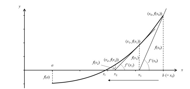
Process of approaching the root x = xr for equation f(x) = 0 by Newton's method
The root crossing the x-axis for equation f(x) = 0 in Example 1
Two roots crossing the x-axis for equation f(x) = 0 in Example 2
The graph of the function in range [0.5, 1] in Example 4 (red) and the tangent line crossing the right endpoint (1, 0.1585) in blue and that crossing point (0.5, –0.2294) in green
The graph of the function in range [0, 1.5] in Example 5 (red) and the tangent line crossing the right endpoint (1.5 0.5975) in blue and that crossing point (1, 0.3415) in green