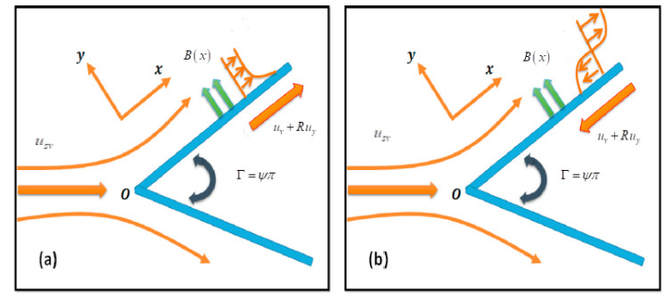
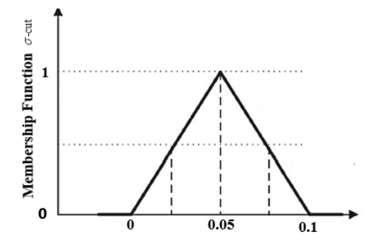
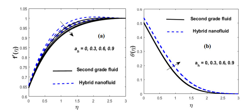
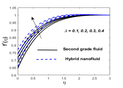
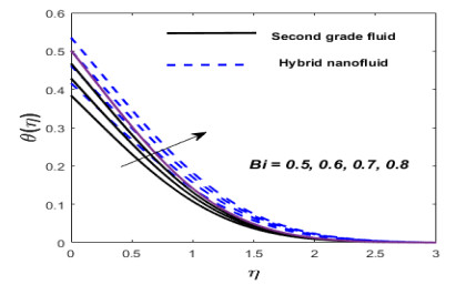
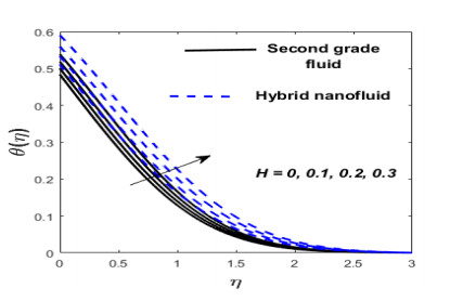
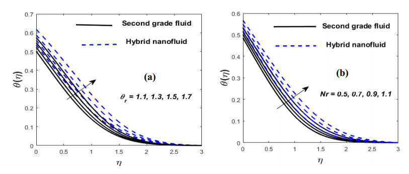
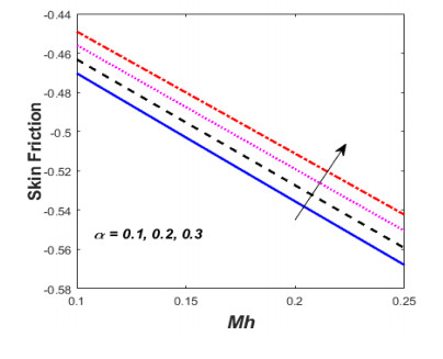
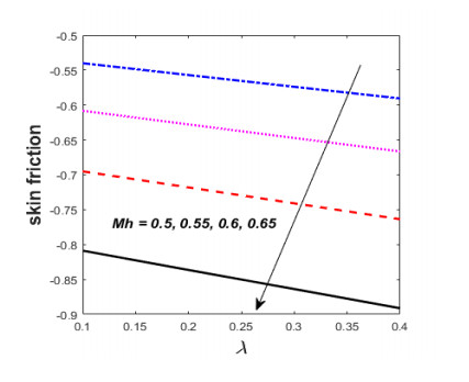
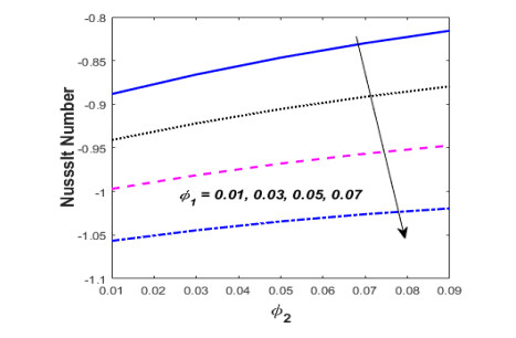
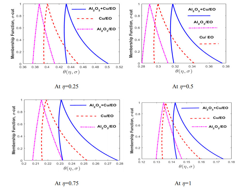
This investigation presents the fuzzy nanoparticle volume fraction on heat transfer of second-grade hybrid $ {\text{A}}{{\text{l}}_{\text{2}}}{{\text{O}}_{\text{3}}}{\text{ + Cu/EO}} $ nanofluid over a stretching/shrinking Riga wedge under the contribution of heat source, stagnation point, and nonlinear thermal radiation. Also, this inquiry includes flow simulations using modified Hartmann number, boundary wall slip and heat convective boundary condition. Engine oil is used as the host fluid and two distinct nanomaterials ($ {\text{Cu}} $ and $ {\text{A}}{{\text{l}}_{\text{2}}}{{\text{O}}_{\text{3}}} $) are used as nanoparticles. The associated nonlinear governing PDEs are intended to be reduced into ODEs using suitable transformations. After that 'bvp4c, ' a MATLAB technique is used to compute the solution of said problem. For validation, the current findings are consistent with those previously published. The temperature of the hybrid nanofluid rises significantly more quickly than the temperature of the second-grade fluid, for larger values of the wedge angle parameter, the volume percentage of nanomaterials. For improvements to the wedge angle and Hartmann parameter, the skin friction factor improves. Also, for the comparison of nanofluids and hybrid nanofluids through membership function (MF), the nanoparticle volume fraction is taken as a triangular fuzzy number (TFN) in this work. Membership function and $ \sigma {\text{ - cut}} $ are controlled TFN which ranges from 0 to 1. According to the fuzzy analysis, the hybrid nanofluid gives a more heat transfer rate as compared to nanofluids. Heat transfer and boundary layer flow at wedges have recently received a lot of attention due to several metallurgical and engineering physical applications such as continuous casting, metal extrusion, wire drawing, plastic, hot rolling, crystal growing, fibreglass and paper manufacturing.
Citation: Imran Siddique, Yasir Khan, Muhammad Nadeem, Jan Awrejcewicz, Muhammad Bilal. Significance of heat transfer for second-grade fuzzy hybrid nanofluid flow over a stretching/shrinking Riga wedge[J]. AIMS Mathematics, 2023, 8(1): 295-316. doi: 10.3934/math.2023014
This investigation presents the fuzzy nanoparticle volume fraction on heat transfer of second-grade hybrid $ {\text{A}}{{\text{l}}_{\text{2}}}{{\text{O}}_{\text{3}}}{\text{ + Cu/EO}} $ nanofluid over a stretching/shrinking Riga wedge under the contribution of heat source, stagnation point, and nonlinear thermal radiation. Also, this inquiry includes flow simulations using modified Hartmann number, boundary wall slip and heat convective boundary condition. Engine oil is used as the host fluid and two distinct nanomaterials ($ {\text{Cu}} $ and $ {\text{A}}{{\text{l}}_{\text{2}}}{{\text{O}}_{\text{3}}} $) are used as nanoparticles. The associated nonlinear governing PDEs are intended to be reduced into ODEs using suitable transformations. After that 'bvp4c, ' a MATLAB technique is used to compute the solution of said problem. For validation, the current findings are consistent with those previously published. The temperature of the hybrid nanofluid rises significantly more quickly than the temperature of the second-grade fluid, for larger values of the wedge angle parameter, the volume percentage of nanomaterials. For improvements to the wedge angle and Hartmann parameter, the skin friction factor improves. Also, for the comparison of nanofluids and hybrid nanofluids through membership function (MF), the nanoparticle volume fraction is taken as a triangular fuzzy number (TFN) in this work. Membership function and $ \sigma {\text{ - cut}} $ are controlled TFN which ranges from 0 to 1. According to the fuzzy analysis, the hybrid nanofluid gives a more heat transfer rate as compared to nanofluids. Heat transfer and boundary layer flow at wedges have recently received a lot of attention due to several metallurgical and engineering physical applications such as continuous casting, metal extrusion, wire drawing, plastic, hot rolling, crystal growing, fibreglass and paper manufacturing.

| [1] |
G. Rasool, T. Zhang, A. Shafiq, Second grade nanofluidic fow past a convectively heated vertical Riga plate, Phys. Scr., 12 (2019), 125212. https://doi.org/10.1088/1402-4896/ab3990 doi: 10.1088/1402-4896/ab3990

|
| [2] |
T. Abbas, M. Ayub, M. M. Bhatti, M. M. Rashidi, M. E. Ali, Entropy generation on nanofuid fow through a horizontal Riga-plate, Entropy, 18 (2016), 223. https://doi.org/10.3390/e18060223 doi: 10.3390/e18060223
|
| [3] | A. B. Tsinober, A. G. Shtern, Possibility of increasing the flow stability in a boundary layer using crossed electric and magnetic fields, Magnetohydrodynamics, 3 (1967), 103–105. |
| [4] |
S. Abdal, I. Siddique, A. S. Alshomrani, F. Jarad, I. S. U. Din, S. Afzal, Significance of chemical reaction with activation energy for Riga wedge flow of tangent hyperbolic nanofluid in existence of heat source, Case Stud. Therm. Eng., 28 (2021), 101542. https://doi.org/10.1016/j.csite.2021.101542 doi: 10.1016/j.csite.2021.101542
|
| [5] |
K. Gangadhar, M. A. Kumari, A. J. Chamkha, EMHD flow of radiative second-grade nanofluid over a Riga plate due to convective heating: Revised Buongiorno's nanofluid model, Arab. J. Sci. Eng., 2021, 1–11. https://doi.org/10.1007/s13369-021-06092-7 doi: 10.1007/s13369-021-06092-7
|
| [6] |
M. I. Khan, F. Alzahrani, Dynamics of viscoelastic fluid conveying nanoparticles over a wedge when bioconvection and melting process are significant, Int. Commun. Heat Mass, 128 (2021), 105604. https://doi.org/10.1016/j.icheatmasstransfer.2021.105604 doi: 10.1016/j.icheatmasstransfer.2021.105604
|
| [7] |
D. Vieru, I. Siddique, M. Kamran, C. Fetecau, Energetic balance for the flow of a second-grade fluid due to a plate subject to shear stress, Comput. Math. Appl., 4 (2008), 1128–1137. https://doi.org/10.1016/j.camwa.2008.02.013 doi: 10.1016/j.camwa.2008.02.013
|
| [8] | A. Mahmood, C. Fetecau, I. Siddique, Exact solutions for some unsteady flows of generalized second grade fluids in cylindrical domains, J. Prim. Res. Math., 4 (2008), 171–180. Available from: http://www.sms.edu.pk/jprm/media/pdf/jprm/volume_04/jprm10_4.pdf |
| [9] |
M. Ramzan, M. Bilal, Time-dependent MHD nano-second grade fluid flow induced by a permeable vertical sheet with mixed convection and thermal radiation, PLoS One, 10 (2015). https://doi.org/10.1371/journal.pone.0124929 doi: 10.1371/journal.pone.0124929
|
| [10] |
M. Ramzan, M. Bilal, U. Farooq, J. D. Chung, Mixed convective radiative flow of second grade nanofluid with convective boundary conditions: an optimal solution, Res. Phys., 6 (2016), 796–804. https://doi.org/10.1016/j.rinp.2016.10.011 doi: 10.1016/j.rinp.2016.10.011
|
| [11] | S. K. Rawat, H. Upreti, M. Kumar, Comparative study of mixed convective MHD Cu-water nanofluid flow over a cone and wedge using modified Buongiorno's model in presence of thermal radiation and chemical reaction via Cattaneo-Christov double diffusion model, J. Appl. Comput. Mech., 2020. Available from: https://jacm.scu.ac.ir/article_15395_9ede39b5e33cc127967e197282afed32. |
| [12] |
S. Rajput, A. K. Verma, K. Bhattacharyya, A. J. Chamkha, Unsteady nonlinear mixed convective flow of nanofluid over a wedge: Buongiorno model, Waves Random Complex, 2021, 1–15. https://doi.org/10.1080/17455030.2021.1987586 doi: 10.1080/17455030.2021.1987586
|
| [13] |
A. Mishra, M. Kumar, Numerical analysis of MHD nanofluid flow over a wedge, including effects of viscous dissipation and heat generation/absorption, using Buongiorno model, Heat Transfer, 8 (2021), 8453–8474. https://doi.org/10.1002/htj.22284 doi: 10.1002/htj.22284
|
| [14] |
R. Garia, S. K. Rawat, M. Kumar, M. Yaseen, Hybrid nanofluid flow over two different geometries with Cattaneo-Christov heat flux model and heat generation: A model with correlation coefficient and probable error, Chinese J. Phys., 74 (2021), 421–439. https://doi.org/10.1016/j.cjph.2021.10.030 doi: 10.1016/j.cjph.2021.10.030
|
| [15] | I. Siddique, M. Nadeem, J. Awrejcewicz, W. Pawłowski, Soret and Dufour effects on unsteady MHD second-grade nanofluid flow across an exponentially stretching surface, Sci Rep., 12 (2022), 11811. https://www.nature.com/articles/s41598-022-16173-8 |
| [16] | S. U. Choi, J. A. Eastman, Enhancing thermal conductivity of fluids with nanoparticles (No. ANL/MSD/CP-84938; CONF-951135-29), Argonne National Lab., IL (United States), 1995. Available from: https://ecotert.com/pdf/196525_From_unt-edu.pdf |
| [17] |
S. Suresh, K. P. Venkitaraj, P. Selvakumar, Effect of Al2O3-Cu/water hybrid nanofluid in heat transfer, Exp. Therm. Fluid Sci., 38 (2012), 54–60. https://doi.org/10.1016/j.expthermflusci.2011.11.007 doi: 10.1016/j.expthermflusci.2011.11.007
|
| [18] |
L. S. Sundar, A. C. Sousa, M. K. Singh, Heat transfer enhancement of low volume concentration of carbon nanotube-Fe3O4/water hybrid nanofluids in a tube with twisted tape inserts under turbulent flow, J. Therm. Sci. Eng. Appl., 7 (2015), 021015. https://doi.org/10.1115/1.4029622 doi: 10.1115/1.4029622
|
| [19] |
S. Nadeem, N. Abbas, A. U. Khan, Characteristics of three dimensional stagnation point flow of Hybrid nanofluid past a circular cylinder, Results Phys., 8 (2018), 829–835. https://doi.org/10.1016/j.rinp.2018.01.024 doi: 10.1016/j.rinp.2018.01.024
|
| [20] |
S. Nadeem, N. Abbas, On both MHD and slip effect in micropolar hybrid nanofluid past a circular cylinder under stagnation point region, Can. J. Phys., 97 (2018), 392–399. https://doi.org/10.1139/cjp-2018-017 doi: 10.1139/cjp-2018-017
|
| [21] |
S. Yan, D. Toghraie, L. A. Abdulkareem, A. Alizadeh, P. Barnoon, M. Afrand, The rheological behavior of MWCNTs-ZnO/water-ethylene glycol hybrid non-Newtonian nanofluid by using of an experimental investigation, J. Mater. Res. Technol., 9 (2020), 8401–8406. https://doi.org/10.1016/j.jmrt.2020.05.018 doi: 10.1016/j.jmrt.2020.05.018
|
| [22] |
A. U. Rehman, R. Mehmood, S. Nadeem, N. S. Akbar, S. S. Motsa, Effects of single and multi-walled carbon nano tubes on water and engine oil based rotating fluids with internal heating, Adv. Powder Technol., 28 (2017), 1991–2002. https://doi.org/10.1016/j.apt.2017.03.017 doi: 10.1016/j.apt.2017.03.017
|
| [23] |
N. A. L. Aladdin, N. Bachok, I. Pop, Cu-Al2O3/water hybrid nanofluid flow over a permeable moving surface in presence of hydromagnetic and suction effects, Alex. Eng. J., 59 (2020), 657–666. https://doi.org/10.1016/j.aej.2020.01.028 doi: 10.1016/j.aej.2020.01.028
|
| [24] |
N. S. Anuar, N. Bachok, N. M. Arifin, H. Rosali, Analysis of Al2O3-Cu nanofluid flow behaviour over a permeable moving wedge with convective surface boundary conditions, J. King Saud Univ. Sci., 33 (2021), 101370. https://doi.org/10.1016/j.jksus.2021.101370 doi: 10.1016/j.jksus.2021.101370
|
| [25] | M. Nadeem, I. Siddique, J. Awrejcewicz, M. Bilal, Numerical analysis of a second-grade fuzzy hybrid nanofluid flow and heat transfer over a permeable stretching/shrinking sheet, Sci. Rep.-UK, 12 (2022), 1–17. https://www.nature.com/articles/s41598-022-05393-7 |
| [26] |
N. Joshi, A. K. Pandey, H. Upreti, M. Kumar, Mixed convection flow of magnetic hybrid nanofluid over a bidirectional porous surface with internal heat generation and a higher‐order chemical reaction, Heat Transfer, 50 (2021), 3661–3682. https://doi.org/10.1002/htj.22046 doi: 10.1002/htj.22046
|
| [27] | N. Joshi, H. Upreti, A. K. Pandey, M. Kumar, Heat and mass transfer assessment of magnetic hybrid nanofluid flow via bidirectional porous surface with volumetric heat generation, Int. J. Appl. Comput. Math., 7 (2021), 1–17. Available from: https://link.springer.com/article/10.1007/s40819-021-00999-3 |
| [28] | T. Watanabe, Thermal boundary layers over a wedge with uniform suction or injection in forced flow, Acta Mech., 83 (1990), 119–126. Available from: https://link.springer.com/article/10.1007/BF01172973 |
| [29] |
N. A. Yacob, A. Ishak, I. Pop, Falkner-Skan problem for a static or moving wedge in nanofluids, Int. J. Therm. Sci., 50 (2011), 133–139. https://doi.org/10.1016/j.ijthermalsci.2010.10.008 doi: 10.1016/j.ijthermalsci.2010.10.008
|
| [30] |
H. Upreti, A. K. Pandey, M. Kumar, Assessment of entropy generation and heat transfer in three-dimensional hybrid nanofluids flow due to convective surface and base fluids, J. Porous Media, 24 (2021). https://doi.org/10.1615/JPorMedia.2021036038 doi: 10.1615/JPorMedia.2021036038
|
| [31] | A. Mishra, M. Kumar, Velocity and thermal slip effects on MHD nanofluid flow past a stretching cylinder with viscous dissipation and Joule heating, SN Appl. Sci., 2 (2020), 1–13. Available from: https://link.springer.com/article/10.1007/s42452-020-3156-7. |
| [32] |
A. Mishra, H. Upreti, A comparative study of Ag-MgO/water and Fe3O4-CoFe2O4/EG-water hybrid nanofluid flow over a curved surface with chemical reaction using Buongiorno model, Partial Differ. Eq. Appl. Math., 5 (2022), 100322, 2666–8181. https://doi.org/10.1016/j.padiff.2022.100322 doi: 10.1016/j.padiff.2022.100322
|
| [33] | M. Yaseen, S. K. Rawat, M. Kumar, Cattaneo-Christov heat flux model in Darcy-Forchheimer radiative flow of MoS2-SiO2/kerosene oil between two parallel rotating disks, J. Therm. Anal. Calorim., 2022, 1–23. Available from: https://link.springer.com/article/10.1007/s10973-022-11248-0. |
| [34] | S. K. Rawat, M. Kumar, Cattaneo-Christov heat flux model in flow of copper water nanofluid through a stretching/shrinking sheet on stagnation point in presence of heat generation/absorption and activation energy, Int. J. Appl. Comput. Math., 6 (2020), 1–26. Available from: https://link.springer.com/article/10.1007/s40819-020-00865-8. |
| [35] | A. Gailitis, O. Lielausis, On possibility to reduce the hydrodynamics resistance of a plate in an electrolyte, Appl. Magn. Rep. Phys. Inst. Riga, 12 (1961), 143–146. Available from: https://scirp.org/reference/ReferencesPapers.aspx?ReferenceID=1927365. |
| [36] |
H. T. Basha, R. Sivaraj, I. L. Animasaun, Stability analysis on Ag-MgO/water hybrid nanofluid flow over an extending/contracting Riga wedge and stagnation point, CTS, 12 (2020), 6. https://doi.org/10.1615/ComputThermalScien.2020034373 doi: 10.1615/ComputThermalScien.2020034373
|
| [37] | G. Rasool, A. Wakif, Numerical spectral examination of EMHD mixed convection flow of second-grade nanofluid towards a vertical Riga plate used an advanced version of the revised Buongiorno's nanofluid model, J. Therm. Anal. Calorim., 143 (2021), 2379–2393. Available from: https://link.springer.com/article/10.1007/s10973-020-09865-8. |
| [38] | G. K. Ramesh, G. S. Roopa, B. J. Gireesha, S. A. Shehzad, F. M. Abbasi, An electro-magneto-hydrodynamic flow Maxwell nanoliquid past a Riga plate: A numerical study, J. Brazilian Soc. Mech. Sci. Eng., 39 (2017), 4547–4554. Available from: https://link.springer.com/article/10.1007/s40430-017-0900-z. |
| [39] |
A. Shafiq, I. Zari, I. Khan, T. S. Khan, A. H. Seikh, E. S. M. Sherif, Marangoni driven boundary layer flow of carbon nanotubes toward a Riga plate, Front. Phys., 7 (2020), 1–11. https://doi.org/10.3389/fphy.2019.00215 doi: 10.3389/fphy.2019.00215
|
| [40] |
N. Ahmed, Adnan, U. Khan, S. T. Mohyud-Din, Influence of thermal radiation and viscous dissipation on squeezed flow of water between Riga plates saturated with carbon nanotubes, Colloid. Surface. A., 522 (2017), 389–398. https://doi.org/10.1016/j.colsurfa.2017.02.083 doi: 10.1016/j.colsurfa.2017.02.083
|
| [41] |
M. Ayub, T. Abbas, M. M. Bhatti, Inspiration of slip effects on EMHD nanofluid flow through a horizontal Riga plate, Eur. Phys. J. Plus, 131 (2016), 1–9. https://doi.org/10.1140/epjp/i2016-16193-4 doi: 10.1140/epjp/i2016-16193-4
|
| [42] |
A. Zaib, R. U. Haq, A. J. Chamkha, M. M. Rashidi, Impact of partial slip on mixed convective flow towards a Riga plate comprising micropolar TiO2-kerosene/water nanoparticles, Int. J. Numer. Meth. H., 29 (2018), 1647–1662. https://doi.org/10.1108/HFF-06-2018-0258 doi: 10.1108/HFF-06-2018-0258
|
| [43] |
T. Abbas, M. Ayub, M. M. Bhatti, M. M. Rashidi, M. E. S. Ali, Entropy generation on nanofluid flow through a horizontal Riga plate, Entropy, 18 (2016), 223. https://doi.org/10.3390/e18060223 doi: 10.3390/e18060223
|
| [44] |
M. M. Bhatti, T. Abbas, M. M. Rashidi, Effects of thermal radiation and electro magneto hydrodynamics on viscous nanofluid through a Riga plate, Multidiscip. Model. Ma., 12 (2016), 605–618. https://doi.org/10.1108/MMMS-07-2016-0029 doi: 10.1108/MMMS-07-2016-0029
|
| [45] |
E. Magyari, A. Pantokratoras, Aiding and opposing mixed convection flows over the Riga-plate, Commun. Nonlinear Sci. Numer. Simul., 16 (2011), 3158–3167. https://doi.org/10.1016/j.cnsns.2010.12.003 doi: 10.1016/j.cnsns.2010.12.003
|
| [46] |
J. Pang, K. S. Choi, Turbulent drag reduction by Lorentz force oscillation, Phys. Fluids, 16 (2004). https://doi.org/10.1063/1.1689711 doi: 10.1063/1.1689711
|
| [47] |
Y. Liu, Y. Jian, W. Tan, Entropy generation of electromagnetohydrodynamic (EMHD) flow in a curved rectangular microchannel, Int. J. Heat Mass Transf., 127 (2018), 901–913. https://doi.org/10.1016/j.ijheatmasstransfer.2018.06.147 doi: 10.1016/j.ijheatmasstransfer.2018.06.147
|
| [48] |
N. A. Zainal, R. Nazar, K. Naganthran, I. Pop, Unsteady EMHD stagnation point flow over a stretching/shrinking sheet in a hybrid Al2O3-Cu/H2O nanofluid, Int. Commun. Heat Mass, 123 (2021), 105205. https://doi.org/10.1016/j.icheatmasstransfer.2021.105205 doi: 10.1016/j.icheatmasstransfer.2021.105205
|
| [49] |
M. Bilal, Micropolar flow of EMHD nanofluid with nonlinear thermal radiation and slip effects, Alex. Eng. J., 59 (2020), 965–976. https://doi.org/10.1016/j.aej.2020.03.023 doi: 10.1016/j.aej.2020.03.023
|
| [50] |
N. Kakar, A. Khalid, A. S. Al-Johani, N. Alshammari, I. Khan, Melting heat transfer of a magnetized water-based hybrid nanofluid flow past over a stretching/shrinking wedge, Case Stud. Therm. Eng., 30 (2022), 101674. https://doi.org/10.1016/j.csite.2021.101674 doi: 10.1016/j.csite.2021.101674
|
| [51] | T. Abbas, T. Hayat, M. Ayub, M. M. Bhatti, A. Alsaedi, Electromagnetohydrodynamic nanofluid flow past a porous Riga plate containing gyrotactic microorganism, Neural Comput. Appl., 31 (2019), 1905–1913. Available from: https://link.springer.com/article/10.1007/s00521-017-3165-7. |
| [52] |
N. Joshi, H. Upreti, A. K. Pandey, MHD Darcy-Forchheimer Cu-Ag/H2O-C2H6O2 hybrid nanofluid flow via a porous stretching sheet with suction/blowing and viscous dissipation, Int. J. Comput. Meth. Eng. Sci. Mech., 2022, 1–9. https://doi.org/10.1080/15502287.2022.2030426 doi: 10.1080/15502287.2022.2030426
|
| [53] |
A. Mishra, H. Upreti, A comparative study of Ag-MgO/water and Fe3O4-CoFe2O4/EG-water hybrid nanofluid flow over a curved surface with chemical reaction using Buongiorno model, Partial Differ. Eq. Appl. Math., 5 (2022), 100322. https://doi.org/10.1016/j.padiff.2022.100322 doi: 10.1016/j.padiff.2022.100322
|
| [54] | S. Abdal, U. Habib, I. Siddique, A. Akgül, B. Ali, Attribution of multi-slips and bioconvection for micropolar nanofluids transpiration through porous medium over an extending sheet with PST and PHF conditions, Int. J. Appl. Comput. Math., 7 (2021), 1–21. Available from: https://link.springer.com/article/10.1007/s40819-021-01137-9. |
| [55] | S. Abdal, I. Siddique, D. Alrowaili, Q. Al-Mdallal, S. Hussain, Exploring the magnetohydrodynamic stretched flow of Williamson Maxwell nanofluid through porous matrix over a permeated sheet with bioconvection and activation energy, Sci. Rep., 12 (2022), 1–12. Available from: https://www.nature.com/articles/s41598-021-04581-1. |
| [56] |
L. A. Zadeh, Fuzzy sets, Inform. Control, 8 (1965), 338–353. https://doi.org/10.1142/9789814261302_0021 doi: 10.1142/9789814261302_0021
|
| [57] |
S. Chang, L. Zadeh, On fuzzy mapping and control, IEEE T. Syst. Man Cy., 2 (1972), 30–34. https://doi.org/10.1109/TSMC.1972.5408553 doi: 10.1109/TSMC.1972.5408553
|
| [58] |
D. Dubois, H. Prade, Towards fuzzy differential calculus: part 3, differentiation, Fuzzy Set. Syst., 8 (1982), 30–34. https://doi.org/10.1016/S0165-0114(82)80001-8 doi: 10.1016/S0165-0114(82)80001-8
|
| [59] |
O. Kaleva, Fuzzy differential equations, Fuzzy Set. Syst., 24 (1987), 301–307. https://doi.org/10.1016/0165-0114(87)90029-7 doi: 10.1016/0165-0114(87)90029-7
|
| [60] |
O. Kaleva, The cauchy problem for fuzzy differential equations, Fuzzy Set. Syst., 24 (1990), 389–396. https://doi.org/10.1016/0165-0114(90)90010-4 doi: 10.1016/0165-0114(90)90010-4
|
| [61] |
S. Seikkala, On the fuzzy initial value problem, Fuzzy Set. Syst., 24 (1987), 319–330. https://doi.org/10.1016/0165-0114(87)90030-3 doi: 10.1016/0165-0114(87)90030-3
|
| [62] |
G. Borah, P. Dutta, G. C. Hazarika, Numerical study on second-grade fluid flow problems using analysis of fractional derivatives under fuzzy environment, Soft Comput. Tech. Appl. Adv. Intell. Syst. Comput. 1248 (2021). https://doi.org/10.1007/978-981-15-7394-1_4 doi: 10.1007/978-981-15-7394-1_4
|
| [63] |
A. Barhoi, G. C. Hazarika, P. Dutta, Numerical solution of MHD Viscous flow over a shrinking sheet with second order slip under fuzzy environment, Adv. Math. Sci. J., 9 (2020), 10621–10631. https://doi.org/10.37418/amsj.9.12.47 doi: 10.37418/amsj.9.12.47
|
| [64] |
U. Biswal, S. Chakraverty, B. K. Ojha, Natural convection of nanofluid flow between two vertical flat plates with imprecise parameter, Coupled Syst. Mech., 9 (2020), 219–235. https://doi.org/10.12989/csm.2020.9.3.219 doi: 10.12989/csm.2020.9.3.219
|
| [65] |
M. Nadeem, A. Elmoasry, I. Siddique, F. Jarad, R. M. Zulqarnain, J. Alebraheem, N. S. Elazab, Study of triangular fuzzy hybrid nanofluids on the natural convection flow and heat transfer between two vertical plates, Comput. Intell. Neurosc., 2021 (2021). https://doi.org/10.1155/2021/3678335 doi: 10.1155/2021/3678335
|
| [66] |
I. Siddique, R. M. Zulqarnain, M. Nadeem, F. Jarad, Numerical simulation of MHD Couette flow of a fuzzy nanofluid through an inclined channel with thermal radiation effect, Comput. Intell. Neurosc., 2021 (2021), 1–16. https://doi.org/10.1155/2021/6608684 doi: 10.1155/2021/6608684
|
| [67] | S. Chakraverty, S. Tapaswini, D. Behera, Fuzzy differential equations and applications for engineers and scientists, CRC Press, Boca Raton, 2016. https://doi.org/10.1201/9781315372853 |
| [68] |
M. Nadeem, I. Siddique, R. Ali, N. Alshammari, R. N. Jamil, N. Hamadneh, M. Andualem, Study of third-grade fluid under the fuzzy environment with Couette and Poiseuille flows, Math. Probl. Eng., 2022 (2022). https://doi.org/10.1155/2022/2458253 doi: 10.1155/2022/2458253
|
| [69] |
I. Siddique, R. M. Zulqarnain, M. Nadeem, F. Jarad, Numerical simulation of mhd couette flow of a fuzzy nanofluid through an inclined channel with thermal radiation effect, Comput. Intell. Neurosc., 2021 (2021). https://doi.org/10.1155/2021/6608684 doi: 10.1155/2021/6608684
|
| [70] |
M. Nadeem, I. Siddique, F. Jarad, R. N. Jamil, Numerical study of MHD third-grade fluid flow through an inclined channel with ohmic heating under fuzzy environment, Math. Probl. Eng., 2021 (2021). https://doi.org/10.1155/2021/9137479 doi: 10.1155/2021/9137479
|
| [71] |
M. Bilal, H. Tariq, Y. Urva, I. Siddique, S. Shah, T. Sajid, et al., A novel nonlinear diffusion model of magneto-micropolar fluid comprising Joule heating and velocity slip effects, Wave. Random Complex, 2022, 1–17. https://doi.org/10.1080/17455030.2022.2079761 doi: 10.1080/17455030.2022.2079761
|
| [72] |
I. Siddique, R. N. Jamil, M. Nadeem, H. A. El-Wahed Khalifa, F. Alotaibi, I. Khan, et al., Fuzzy analysis for thin-film flow of a third-grade fluid down an inclined plane, Math. Probl. Eng., 2022 (2022), 3495228. https://doi.org/10.1155/2022/3495228 doi: 10.1155/2022/3495228
|
| [73] | I. Siddique, M. Nadeem, I. Khan, R. N. Jamil, M. A. Shamseldin, A. Akgül, Analysis of fuzzified boundary value problems for MHD Couette and Poiseuille flow, Sci. Rep.-UK, 12 (2022), 1–28. Available from: https://www.nature.com/articles/s41598-022-12110-x. |
Figures(16) / Tables(4)

Imran Siddique, Yasir Khan, Muhammad Nadeem, Jan Awrejcewicz, Muhammad Bilal. Significance of heat transfer for second-grade fuzzy hybrid nanofluid flow over a stretching/shrinking Riga wedge[J]. AIMS Mathematics, 2023, 8(1): 295-316. doi: 10.3934/math.2023014


 DownLoad: