Geriatrics as an educational topic has been a high priority in current health care. The innovative Age-Friendly health system with the 4Ms structure (what Matters most, Medication, Mentation, Mobility) needs to be integrated into oral health and dental services training. The purpose of this study is to respond to one question: are the graduating general dentists trained and prepared to treat medically vulnerable elderly in communities?
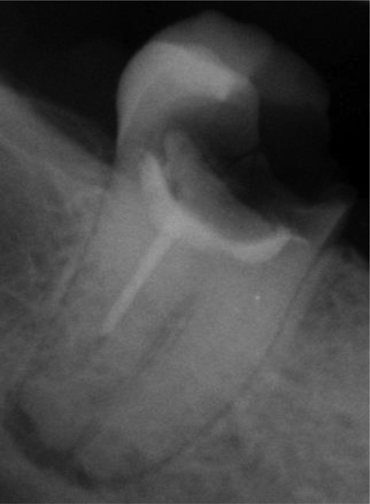
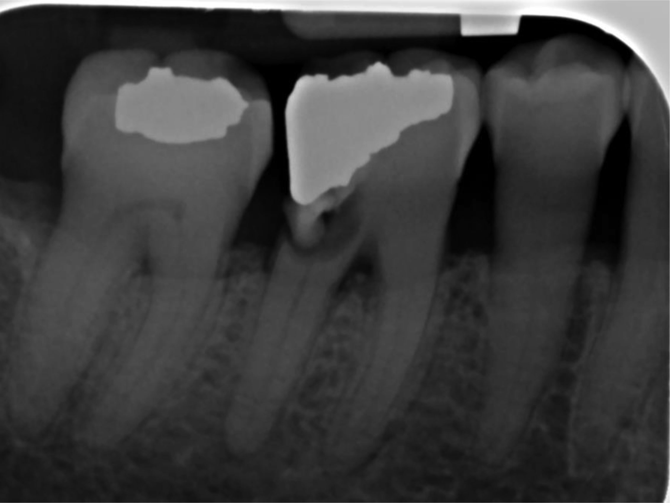
All pre-doctorate dental students from first year to fourth year were invited to voluntarily respond to an online survey provided on Qualtrics. The survey provided examples of two broken molar teeth that need extraction. First, students were asked how comfortable they felt extracting the two molars based on the x-rays. Then, the question was repeated to evaluate if they felt comfortable with extracting the teeth in a patient with one chronic condition and related medication(s). Finally, the students were again questioned whether they feel comfortable to provide the same service to medically vulnerable patients with multiple health conditions and polypharmacy.
The majority of students who participated in this study said they were comfortable with extracting the teeth of patients without any chronic condition. However, many more chose to refer medically vulnerable patients with multiple chronic conditions and polypharmacy to a specialist.
Dental education in many U.S. dental schools may provide adequate education and create competent general dentists. Yet, the competency and confidence required for dentists to be able to treat older adults with multiple health conditions and using prescribed or over-the-counter medication is insufficient.
Citation: Maryam Tabrizi, Wei-Chen Lee. Geriatric oral health competency among dental providers[J]. AIMS Public Health, 2021, 8(4): 682-690. doi: 10.3934/publichealth.2021054
Geriatrics as an educational topic has been a high priority in current health care. The innovative Age-Friendly health system with the 4Ms structure (what Matters most, Medication, Mentation, Mobility) needs to be integrated into oral health and dental services training. The purpose of this study is to respond to one question: are the graduating general dentists trained and prepared to treat medically vulnerable elderly in communities?
All pre-doctorate dental students from first year to fourth year were invited to voluntarily respond to an online survey provided on Qualtrics. The survey provided examples of two broken molar teeth that need extraction. First, students were asked how comfortable they felt extracting the two molars based on the x-rays. Then, the question was repeated to evaluate if they felt comfortable with extracting the teeth in a patient with one chronic condition and related medication(s). Finally, the students were again questioned whether they feel comfortable to provide the same service to medically vulnerable patients with multiple health conditions and polypharmacy.
The majority of students who participated in this study said they were comfortable with extracting the teeth of patients without any chronic condition. However, many more chose to refer medically vulnerable patients with multiple chronic conditions and polypharmacy to a specialist.
Dental education in many U.S. dental schools may provide adequate education and create competent general dentists. Yet, the competency and confidence required for dentists to be able to treat older adults with multiple health conditions and using prescribed or over-the-counter medication is insufficient.

| [1] | Colby SL, Ortman JM Projections of the size and composition of the U.S. population: 2014 to 2060 (2015). Available from: https://www.census.gov/content/dam/Census/library/publications/2015/demo/p25-1143.pdf. |
| [2] |
Fried LP, Hall WJ (2008) Leading on behalf of an aging society. J Am Geriatr Soc 56: 1791-1795. 
|
| [3] | (2017) U.S. Department of Health and Human Services, Health Resources and Services Administration, national Center for Health Workforce AnalysisNational and regional projections of supply and demand for geriatricians: 2013–2025. Rockville, ML: National Center 8. |
| [4] |
Boersma P, Black LI, Ward BW (2020) Prevalence of multiple chronic conditions among US adults, 2018. Prev Chronic Dis 17: 200130.
|
| [5] | Centers for Disease Control and PreventionOlder adult oral health (2021). Available from: https://www.cdc.gov/oralhealth/basics/adult-oral-health/adult_older.htm |
| [6] |
Ettinger RL, Goettsche ZS, Qian F (2017) Predoctoral teaching of geriatric dentistry in U.S. dental schools. J Dent Educ 81: 921-928.
|
| [7] |
Levy N, Goldblatt RS, Reisine S (2013) Geriatrics education in U.S. dental schools: where do we stand, and what improvements should be made?. J Dent Educ 77: 1270-1285.
|
| [8] |
Tabrizi M, Lee WC (2021) A pilot study of an interprofessional program involving dental, medical, nursing, and pharmacy students. Front Public Health 8: 602957.
|
| [9] | Dentistry TodayDental schools now required to train students to treat the disabled (2019). Available from: https://www.dentistrytoday.com/news/industrynews/item/5286-dental-schools-now-required-to-train-students-to-treat-the-disabled |
| [10] | Institute for Healthcare ImprovementAge-Friendly health systems: guide to using the 4Ms in the care of older adults (2020). Available from: http://www.ihi.org/Engage/Initiatives/Age-Friendly-Health-Systems/Documents/IHIAgeFriendlyHealthSystems_GuidetoUsing4MsCare.pdf |
| [11] | Eldercare Workforce AllianceHRSA announces geriatrics academic career awards (2019). Available from: https://eldercareworkforce.org/ewa-news/hrsa-announces-geriatrics-academic-career-awards/ |
| [12] | American Dental EducationSurvey: more Americans want to visit the dentist (2018). Available from: https://www.ada.org/en/publications/ada-news/2018-archive/march/survey-more-americans-want-to-visit-the-dentist |
| [13] | American Dental EducationAging and Dental Health (2021). Available from: https://www.ada.org/en/member-center/oral-health-topics/aging-and-dental-health |
| [14] | American Dental EducationOral health for independent older adults (2021). Available from: https://www.adea.org/publications/Pages/OralHealthforIndependentOlderAdults.aspx |
| [15] | Centers for Medicare and Medicaid ServicesDental services among Medicare beneficiaries: source of payment and out-of-pocket spending (2016). Available from: https://www.cms.gov/Research-Statistics-Data-and-Systems/Research/MCBS/Downloads/DentalDataHighlightMarch2016.pdf |
| [16] |
Fulmer T, Reuben DB, Auerbach J, et al. (2021) Actualizing better health and health care for older adults. Health Aff (Millwood) 40: 219-225.
|
| [17] | American Public Health AssociationNew public health policy statements adopted at APHA 2020 (2020). Available from: https://www.apha.org/news-and-media/news-releases/apha-news-releases/2020/2020-apha-policy-statements |
| [18] |
Marino R, Ghanim A (2013) Teledentistry: a systematic review of the literature. J Telemed Telecare 19: 179-183.
|
| [19] |
Alabdullah JH, Daniel SJ (2018) A systematic review on the validity of teledentistry. Telemed J E Health 24: 639-648.
|
Figures(2) / Tables(3)

Maryam Tabrizi, Wei-Chen Lee. Geriatric oral health competency among dental providers[J]. AIMS Public Health, 2021, 8(4): 682-690. doi: 10.3934/publichealth.2021054


 DownLoad: