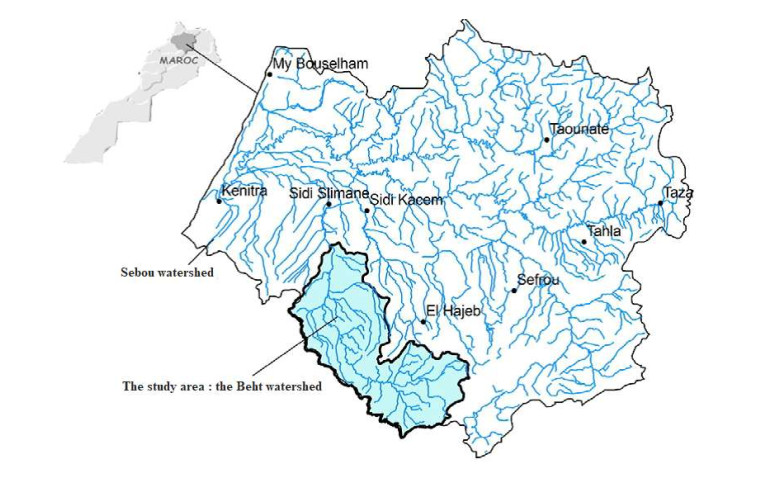
The rocks are likely to give a geochemical signature to the groundwater circulating there. Therefore the hydro geochemistry of the mine's water is influenced by the mining method. The continuous pumping of the mine water gives discharges that induce harmful impacts on the environment. The Sebou basin is subjected to strong industrial and urban pollution, but in the literature, the evaluation of the mining impact on this area is neglected. This paper is dedicated to this issue and as part of the evaluation of the mining impact on the Sebou watershed, the haut Beht mine was chosen among the four mines which include the watershed, and then we proceeded, as the purpose of this work, to evaluate the physicochemical quality of this mine's water discharges and their metallic trace elements (MTE) load (As, Pb, Cd, Zn, and Cu) through monitoring of four locations during two analysis campaigns in 2014 and 2015. This monitoring was performed by ICP-MS analysis. The results showed absenteeism of the acidic nature of mine's water, characterizing acid mine drainage (AMD). The majority of the analyzed water presents important concentrations of sulfate. During the 2014 campaign, the examination of trace metal element concentrations showed, at station 2, contamination of Iron, Aluminum, Manganese and, Arsenic. However, the concentrations of Pb, Cd, Zn, and Cu elements remain conform and very low compared to the limit of standards. The monitoring of the overtake elements made it possible to identify the degree of contamination of the mine's water discharges and to note an improvement in time in the mine water discharges quality.
Citation: Maryem EL FAHEM, Abdellah BENZAOUAK, Habiba ZOUITEN, Amal SERGHINI, Mohamed FEKHAOUI. Hydrogeochemical assessment of mine water discharges from mining activity. Case of the Haut Beht mine (central Morocco)[J]. AIMS Environmental Science, 2021, 8(1): 60-85. doi: 10.3934/environsci.2021005
The rocks are likely to give a geochemical signature to the groundwater circulating there. Therefore the hydro geochemistry of the mine's water is influenced by the mining method. The continuous pumping of the mine water gives discharges that induce harmful impacts on the environment. The Sebou basin is subjected to strong industrial and urban pollution, but in the literature, the evaluation of the mining impact on this area is neglected. This paper is dedicated to this issue and as part of the evaluation of the mining impact on the Sebou watershed, the haut Beht mine was chosen among the four mines which include the watershed, and then we proceeded, as the purpose of this work, to evaluate the physicochemical quality of this mine's water discharges and their metallic trace elements (MTE) load (As, Pb, Cd, Zn, and Cu) through monitoring of four locations during two analysis campaigns in 2014 and 2015. This monitoring was performed by ICP-MS analysis. The results showed absenteeism of the acidic nature of mine's water, characterizing acid mine drainage (AMD). The majority of the analyzed water presents important concentrations of sulfate. During the 2014 campaign, the examination of trace metal element concentrations showed, at station 2, contamination of Iron, Aluminum, Manganese and, Arsenic. However, the concentrations of Pb, Cd, Zn, and Cu elements remain conform and very low compared to the limit of standards. The monitoring of the overtake elements made it possible to identify the degree of contamination of the mine's water discharges and to note an improvement in time in the mine water discharges quality.

| [1] | Ghoreychi M, Laouafa F, Poulard F. L'après-mine et la mécanique des roches; 2017. |
| [2] | Ahmedat C, El hassani I-EEA, Zarhraoui M, et al. (2018) Potentialités minérales et effet de géo-accumulation des éléments traces métalliques des rejets des mines abandonnées. L'exemple des mines d'antimoine de Tourtit et d'Ichoumellal (Maroc central). Bull Inst Sci Rabat 71-89. |
| [3] | Brodkom F (2001) Good Environmental Practice in the European Extractive Industry: A Reference Guide, with Examples from the Industrial Minerals and Gypsum Industries: IMA-Europe. |
| [4] |
Chakraborty P, Gopalapillai Y, Murimboh J, et al. (2006) Kinetic speciation of nickel in mining and municipal effluents. Anal Bioanal Chem 386: 1803-1813. doi: 10.1007/s00216-006-0759-9

|
| [5] | McClure R, Schneider A (2001) The General Mining Act of 1872 has left a legacy of riches and ruin. Seattle Post-Intelligencer 11. |
| [6] | Plumlee GS (1999) The environmental geology of mineral deposits. The environmental geochemistry of mineral deposits Society of Economic Geologists Part A: 71-116. |
| [7] | Touzara S, Amlil A, Ennachete M, et al. (2020) Development of Carbon Paste Electrode/EDTA/Polymer Sensor for Heavy Metals Detection. Anal Bioanal Electrochem 12: 644-652. |
| [8] | Salvarredy Aranguren MM (2008) Contamination en métaux lourds des eaux de surface et des sédiments du Val de Milluni (Andes Boliviennes) par des déchets miniers. Approches géochimique, minéralogique et hydrochimique: Université de Toulouse, Université Toulouse Ⅲ-Paul Sabatier. |
| [9] |
Armiento G, Nardi E, Lucci F, et al. (2017) Antimony and arsenic distribution in a catchment affected by past mining activities: influence of extreme weather events. Rendiconti Lincei 28: 303-315. doi: 10.1007/s12210-016-0566-y
|
| [10] |
Benvenuti M, Mascaro I, Corsini F, et al. (1997) Mine waste dumps and heavy metal pollution in abandoned mining district of Boccheggiano (Southern Tuscany, Italy). Environ Geol 30: 238-243. doi: 10.1007/s002540050152
|
| [11] | Galán E, Gómez-Ariza J, González I, et al. (2003) Heavy metal partitioning in river sediments severely polluted by acid mine drainage in the Iberian Pyrite Belt. Appl. Geochem.Appl Geochem 18: 409-421. |
| [12] |
González RC, González-Chávez M (2006) Metal accumulation in wild plants surrounding mining wastes. Environ Pollut 144: 84-92. doi: 10.1016/j.envpol.2006.01.006
|
| [13] |
Hilton J, Davison W, Ochsenbein U (1985) A mathematical model for analysis of sediment core data: Implications for enrichment factor calculations and trace-metal transport mechanisms. Chem Geol48: 281-291. doi: 10.1016/0009-2541(85)90053-1
|
| [14] |
Jian-Min Z, Zhi D, Mei-Fang C, et al. (2007) Soil heavy metal pollution around the Dabaoshan mine, Guangdong province, China. Pedosphere 17: 588-594. doi: 10.1016/S1002-0160(07)60069-1
|
| [15] | Luoma SN, Rainbow PS (2008) Metal contamination in aquatic environments: science and lateral management: Cambridge university press. |
| [16] |
Mlayah A, Da Silva EF, Rocha F, et al. (2009) The Oued Mellègue: Mining activity, stream sediments and dispersion of base metals in natural environments, North-western Tunisia. J Geochem Explor 102: 27-36. doi: 10.1016/j.gexplo.2008.11.016
|
| [17] | Tessier E (2012) Diagnostic de la contamination sédimentaire par les métaux/métalloï des dans la Rade de Toulon et mécanismes contrô lant leur mobilité. |
| [18] |
Azzaoui s, El hanbali m, Leblanc m (2002) Note technique/Technical Note Cuivre, plomb, fer et manganèse dans le bassin versant du Sebou; Sources d'apport et impact sur la qualité des eaux de surface Copper, Lead, Iron and Manganese in the Sebou.Water qual Res J 37: 773-784. doi: 10.2166/wqrj.2002.052
|
| [19] | Benaabidate L (2000) Caractérisation du bassin versant de Sebou: Hydrologie, Qualité des eaux et géochimie des sources thermales. Docteur Essciences, Univ S MBA, Fès (Maroc) 228. |
| [20] | Foudeil S, BOUNOUIRA H., EMBARCH K., et al. (2013) Evaluation de la pollution en metaux lourds dans l'oued sebou (Maroc). |
| [21] | Foutlane A, Saadallah M, Echihabi L, et al. (2002) Pollution by wastewater for olive oil mills and drinking-water production. Case study of River Sebou in Morocco. |
| [22] | Derwich E, Benaabidate L, Zian A, et al. (2010) Caractérisation physico-chimique des eaux de la nappe alluviale du haut Sebou en aval de sa confluence avec oued Fès. LARHYSS J ISSN 1112-3680. |
| [23] | Derwich E, Beziane Z, Benaabidate L, et al. (2008) Evaluation de la qualité des eaux de surface des Oueds Fès et Sebou utilisées en agriculture maraî chère au Maroc. LARHYSS J ISSN 1112-3680. |
| [24] | Hayzoun H (2014) Caractérisation et quantification de la charge polluante anthropique et industrielle dans le bassin du Sebou. |
| [25] | Lakhili F, Benabdelhadi M, Bouderka N, et al. (2015) Etude de la qualité physicochimique et de la contamination métallique des eaux de surface du bassin versant de Beht (Maroc). Eur Sci J ESJ 11. |
| [26] | Qaouiyid A, Hmima H, Houri K, et al. (2016) Les Teneurs Métalliques Et Paramètres Physico-Chimiques De L'eau Et Du Sédiment De Oued Beht, Au Niveau De Sidi Kacem Et De Oued R'dom Au Niveau De Sidi Slimane. Eur Sci J ESJ 12. |
| [27] | Essamt F (2016) Etude de la qualité d'eau de oued beht dans la région de Sidi Slimane. |
| [28] | Lamhasni N, Chillasse L, Timallouka M (2017) Bio-É valuation De La Qualité Des Eaux De Surface D'oued Beht (Maroc) Indice Biologique Global Des Réseaux De Contrô le Et De Surveillance (IBG-RCS). |
| [29] | Abdallaoui A (1998) Contribution à l'étude du phosphore et des métaux lourds contenus dans les sédiments et de leur influence sur les phénomènes d'eutrophisation et de la pollution: Cas du bassin versant de l'Oued Beht et de la retenue de barrage El Kansera. |
| [30] | Bouchouata O, Ouadarri H, El Abidi A, et al. (2012) Bioaccumulation des métaux lourds par les cultures maraî chères au niveau du Bassin de Sebou (Maroc). Bull Inst Sci Rabat 34: 189-203. |
| [31] | Kenfaoui A (2008) Economisons l'eau en la préservant de la pollution. REV HTE: 140-117. |
| [32] |
Michard A, Soulaimani A, Hoepffner C, et al. (2010) The south-western branch of the Variscan Belt: evidence from Morocco. Tectonophysics 492: 1-24. doi: 10.1016/j.tecto.2010.05.021
|
| [33] |
Piqué A, Michard A (1981) Les zones structurales du Maroc hercynien. Geol Sci Bull Papr 34: 135-146. doi: 10.3406/sgeol.1981.1597
|
| [34] |
Ouabid M, Ouali H, Garrido CJ, et al. (2017) Neoproterozoic granitoids in the basement of the Moroccan Central Meseta: correlation with the Anti-Atlas at the NW paleo-margin of Gondwana. Precambrian Res 299: 34-57. doi: 10.1016/j.precamres.2017.07.007
|
| [35] |
Tahiri A, Montero P, El Hadi H, et al. (2010) Geochronological data on the Rabat-Tiflet granitoids: their bearing on the tectonics of the Moroccan Variscides. J Afr Earth Sci 57: 1-13. doi: 10.1016/j.jafrearsci.2009.07.005
|
| [36] | El Hadi H, Tahiri A, El Maidani A, et al. (2014) Geodynamic setting context of the Permian and Triassic volcanism in the northwestern Moroccan Meseta from petrographical and geochemical data. |
| [37] | Ben Abbou M (1990) Evolution stratigraphique et structurale, au cours du Paléozoï que, de la bordure nord du Massif central (région d'Agourai, Maroc). Unpubl Thesis Univ Fès. |
| [38] | Izart A, Tahiri A, El Boursoumi A, et al. (2001) Carte géologique du Maroc au 1/50 000, feuille de Bouqachmir. Notes et mémoires Serv géol Maroc. |
| [39] | Cailleux Y (1974) Géologie de la région des Smaala (Massif central marocain): stratigraphie du primaire, tectonique hercynienne. |
| [40] | Tahiri A (1994) Tectonique hercynienne de l'anticlinorium de Khouribga-Oulmès et du synclinorium de Fourhal. Bull Inst Sci Rabat 18: 125-144. |
| [41] | Tahiri A, Hoepffner C (1987) La faille d'Oulmès (Maroc central hercynien): cisaillement ductile et tectonique tangentielle. Bull Inst Sci Rabat 11: 59-68. |
| [42] | Sebbag I (1970) Etude géologique et métallogénique de la région du Tafoudeit. Rapport du Service Régional de Géologie-Meknès, service d'étude des gî tes minéraux 29: 62p. |
| [43] | Rassou KK, Razoki B, Yazidi M, et al. (2019) The vulgarization for the patrimonialization of the kettara geodiversity (central jbilet) morocco. |
| [44] | Nerci K (2006) Les minéralisations aurifères du district polymétallique de Tighza (Maroc central): un exemple de mise en place périgranitique tardi-hercynienne. |
| [45] | Giuliani G (1984) Les concentrations filoniennes à tungstène-étain du massif granitique des Zaë r (Maroc Central): minéralisations et phases fluides associées. Mineralium Deposita 19: 193-201. |
| [46] | Salama L, Mouguina EM, Nahid A, et al. (2016) Apport de la modélisation géologique 3D à l'exploration minière: Etude de cas du gisement de Draa Sfar (Jbilets centrales, Maroc)[Mining exploration using 3D geological modeling: Draa Sfar deposit's case study (Central Jbilets, Morocco)]. |
| [47] |
Marcoux E, Belkabir A, Gibson HL, et al. (2008) Draa Sfar, Morocco: A Visean (331 Ma) pyrrhotite-rich, polymetallic volcanogenic massive sulphide deposit in a Hercynian sediment-dominant terrane. Ore Geol Rev 33: 307-328. doi: 10.1016/j.oregeorev.2007.03.004
|
| [48] | Rziki S (2012) Environnement géologique et modèle 3D du gisement polymétallique de Draa Sfar (Massif hercynien des Jebilets, Maroc): Implications et perspectives de développement: Thèse de Doctorat Présentée à la Faculté des Sciences Semlalia Marrakech |
| [49] | DEM Dddm (2011) Les principales mines du maroc. In: Ministère de l'énergie dm, de l'eau et de l'environnement direction du développement minier, editor. É ditions du service géologique du maroc Rabat ed. |
| [50] | Onhym Ondhedm (2020) Oulmes (sn-w) (massif hercynien central, maroc). |
| [51] | Mint chevie M (2010) Contribution à l'étude hydroclimatique du bassin versant de l'Oued Beht, Maroc septentrional. Fès, Maroc: Université Sidi Mohammed Ben Abdellah Faculté des Sciences et Techniques. 58 p. |
| [52] | Burger J, Dardel R, Dutrieux E, et al. (1951) Carte géologique régulière du Maroc au 1: 100.000 eme: Meknès nord, Feuille levée et édifiée par la Société Chérifiènne des Pétroles. Notes et mémoires du Service. |
| [53] | Laabidi A, Gourari L, El hamaidi A (2014) Typologie morpho-sédimentaire des dépô ts actuels de la vallée du Moyen Beht (Sillon sud rifain occidental, Maroc). IOSR J Eng(IOSRJEN) 4. |
| [54] | ABHS AdBHdS (2013) É tude d'actualisation du plan directeur d'aménagement intégré des ressources en eau de bassin hydraulique de Sebou. Note de synthèse, Agence du bassin hydraulique du Sebou. |
| [55] | Duchaufour P (1977) Pédologie: Tome 1: Pédogenèse et classification: Masson. |
| [56] | Bryssine G (1966) Etude des proprietes physiques des dess de l'oued beht. Al Awamia 2: 85-123. |
| [57] | Rachdi HE-N (1995) Etude du volcanisme plio-quaternaire du Maroc central: pétrographie, géochimie et minéralogie: comparaison avec des laves types du Moyen Atlas et du Rekkam (Maroc): Editions du Service géologique du Maroc. |
| [58] | Schmiermund R, Drozd M (1997) Acid mine drainage and other mining-influenced waters (MIW). Mining Environmental Handbook: Effects of Mining on the Environment and American Environmental Controls on Mining: World Scientific. 599-617. |
| [59] | Karim A (2007) Le système siliciclastique-carbonaté de la marge sud-ouest paléotéthysienne au viséen supérieur: enregistrements paléoenvironnementaux et évolution dans un bassin d'avant pays (Tizra: Maroc central): Paris 11. |
| [60] | Pabst T (2011) Etude expérimentale et numérique du comportement hydro-géochimique de recouvrements placés sur des résidus sulfureux partiellement oxydés: Ecole Polytechnique, Montreal (Canada). |
| [61] | Blachere A (1985) Evaluation des impacts hydrogéologiques de l'arrêt d'une exhaure minière (vallées de l'Ondaine et du Lizeron, bassin houiller de la Loire): modélisation mathématique du milieu. |
| [62] | Armines ELEJ-MS (2010) Etat hydrogéochimique et évolution prévisionnelle du site des anciennes exploitations d'uranium de Lodève (Hérault). Centre de Géosciences, É cole des mines de Paris, Fontainebleau, France |
| [63] | El Hachimi ML, EL Hanbali M, Fekhaoui M, et al. (2005) Impact d'un site minier abandonné sur l'environnement: cas de la mine de Zeï da (Haute Moulouya, Maroc). Bull Inst Sci Rabat 93-100. |
| [64] |
Bowell R, Bruce I (1995) Geochemistry of iron ochres and mine waters from Levant Mine, Cornwall. Appl Geochem Appl Geochem10: 237-250. doi: 10.1016/0883-2927(94)00036-6
|
| [65] | Piqué A, Knidiri M (1994) Géologie du Maroc: les domaines régionaux et leur évolution structurale: Pumag. |
| [66] | Taltasse P (1953) Recherches géologiques et hydrogéologiques dans le bassin lacustre de Fès-Meknès: par P. Taltasse: F. Moncho. |
| [67] | Repeta DJ, Quan TM, Aluwihare LI, et al. (2002) Chemical characterization of high molecular weight dissolved organic matter in fresh and marine waters. Geochim. Cosmochim. Acta.66: 955-962. |
| [68] | Debaisieux B (1983) Géologie appliquée à l'aménagement urbain-Saint Etienne(Loire). |
| [69] |
Hackbarth DA (1979) The effects of surface mining of coal on water quality near Grande Cache, Alberta. Can J Earth Sci 16: 1242-1253. doi: 10.1139/e79-109
|
| [70] | Barbier J, Chery L (1997) Relation entre fond géochimique naturel et teneurs élevées en métaux lourds dans les eaux (antimoine, arsenic, baryum, chrome, nickel, plomb, zinc). Rapport BRGM 39544: 51. |
| [71] | Hervé D (1980) Etude de l'acquisition d'une teneur en sulfates par les eaux stockées dans les mines de fer de Lorraine. |
| [72] | Gupta N, Quraishi M, Singh P, et al. (2017) Curcumine longa: Green and sustainable corrosion inhibitor for aluminum in HCl medium. Anal Bioanal Electrochem 9: 245-265. |
| [73] | Marc Fiquet SL, Loic Riou, Bernard Sanjuan (1997) caractérisation des excès d'aluminium dans les eaux superficielles de la martinique. pp. 31. |
| [74] | Kuyucak N (2000) Microorganisms, biotechnology and acid rock drainage—emphasis on passive-biological control and treatment methods. Mining, Metallurgy & Exploration 17: 85-95. |
| [75] | Chatain V (2004) Caractérisation de la mobilisation potentielle de l'arsenic et d'autres constituants inorganiques présents dans les sols issus d'un site minier aurifère: Thèse, Institut National des Sciences Appliquées de Lyon. |
| [76] | Akil A, Hassan T, Lahcen B, et al. (2014) Etude de la qualité physico-chimique et contamination métallique des eaux de surface du bassin versant de Guigou, Maroc. Eur Sci J 10. |
| [77] | Newman DK, Kennedy EK, Coates JD, et al. (1997) Dissimilatory arsenate and sulfate reduction in Desulfotomaculum auripigmentum sp. nov. Arch Microbiol 168: 380-388. |
| [78] | Matera V (2001) Etude de la mobilité et de la spéciation de l'arsenic dans les sols de sites industriels pollués: Estimation du risque induit: Pau. |
| [79] |
Smedley PL, Kinniburgh D (2002) A review of the source, behaviour and distribution of arsenic in natural waters. Appl Geochem 17: 517-568. doi: 10.1016/S0883-2927(02)00018-5
|
| [80] | Laperche V, Bodénan F, Dictor M, et al. (2003) Guide méthodologique de l'arsenic, appliqué à la gestion des sites et sols pollués. Rapport BRGM RP-52066-FR. |
| [81] | Stollenwerk KG (2003) Geochemical processes controlling transport of arsenic in groundwater: a review of adsorption. Arsenic in ground water: Springer. 67-100. |
| [82] |
Cullen WR, Reimer KJ (1989) Arsenic speciation in the environment. Chemical reviews 89: 713-764. doi: 10.1021/cr00094a002
|
| [83] | Inskeep WP, McDernlott TR, Fendorf S (2001) Arsenic (V)/(Ⅲ) Cycling in Soils and Natural Waters: Chemical and Microhiological Processes. Environmental chemistry of arsenic: CRC Press. 203-236. |
| [84] |
Fordham A, Norrish K (1979) Arsenate-73 uptake by components of several acidic soils and its implications for phosphate retention. Soil Research 17: 307-316. doi: 10.1071/SR9790307
|
| [85] |
Livesey N, Huang P (1981) Adsorption of arsenate by soils and its relation to selected chemical properties and anions. Soil Sci131: 88-94. doi: 10.1097/00010694-198102000-00004
|
| [86] |
Bowell R (1994) Sorption of arsenic by iron oxides and oxyhydroxides in soils. Appl Geochem 9: 279-286. doi: 10.1016/0883-2927(94)90038-8
|
| [87] |
Lin Z, Puls R (2000) Adsorption, desorption and oxidation of arsenic affected by clay minerals and aging process. Environ Geol 39: 753-759. doi: 10.1007/s002540050490
|
| [88] |
Grosbois C, Schä fer J, Bril H, et al. (2009) Deconvolution of trace element (As, Cr, Mo, Th, U) sources and pathways to surface waters of a gold mining-influenced watershed. Sci Total Environ 407: 2063-2076. doi: 10.1016/j.scitotenv.2008.11.012
|
| [89] | Bossy A (2010) Origines de l'arsenic dans les eaux, sols et sédiments du district aurifère de S t-Yrieix-la-Perche (Limousin, France): contribution du lessivage des phases porteuses d'arsenic: Université de Tours. |
| [90] |
Shafer MM, Overdier JT, Hurley JP, et al. (1997) The influence of dissolved organic carbon, suspended particulates, and hydrology on the concentration, partitioning and variability of trace metals in two contrasting Wisconsin watersheds (USA). Chem Geol 136: 71-97. doi: 10.1016/S0009-2541(96)00139-8
|
| [91] |
Li X, Shen Z, Wai OW, et al. (2001) Chemical forms of Pb, Zn and Cu in the sediment profiles of the Pearl River Estuary. Marine Mar Pollut Bull 42: 215-223. doi: 10.1016/S0025-326X(00)00145-4
|
| [92] | Morgan JJ, Stumm W (1996) Aquatic chemistry: chemical equilibria and rates in natural waters: Wiley. |
| [93] |
Swedlund P, Webster J (2001) Cu and Zn ternary surface complex formation with SO4 on ferrihydrite and schwertmannite. Appl Geochem 16: 503-511. doi: 10.1016/S0883-2927(00)00044-5
|
| [94] | Aranguren MMS (2008) Contamination en métaux lourds des eaux de surface et des sédiments du Val de Milluni (Andes Boliviennes) par des déchets miniers Approches géochimique, minéralogique et hydrochimique: Université Paul Sabatier-Toulouse Ⅲ. |
| [95] |
Karlsson T, Persson P, Skyllberg U (2005) Extended X-ray absorption fine structure spectroscopy evidence for the complexation of cadmium by reduced sulfur groups in natural organic matter. Environ Sci Technol 39: 3048-3055. doi: 10.1021/es048585a
|
| [96] | Cotton FA, Wilkinson G, Murillo CA, et al. (1988) Advanced inorganic chemistry: Wiley New York. |
| [97] | Ganjali MR, Esmaeili BM, Davarkhah N, et al. (2017) Nano-molar Monitoring of Copper ions in Waste Water Samples by a Novel All-Solid-State Ion Selective Electrode (ASS-ISE). Anal Bioanal Electrochem 9: 187-197. |
| [98] | Bruland K, Lohan M (2006) Controls of trace metals in seawater. The oceans and marine geochemistry 6: 23-47. |
| [99] |
Eary LE (1999) Geochemical and equilibrium trends in mine pit lakes. Appl Geochem 14: 963-987. doi: 10.1016/S0883-2927(99)00049-9
|
| [100] | Baghdad B, Naimi M, Bouabdli A, et al. Evaluation de la contamination et évolution de la qualité des eaux au voisinage d'une mine abandonnée d'extraction de plomb; 2009. |
| [101] | Benzaazoua M (1996) Caractérisation physico-chimique et minéralogique de produits miniers sulfurés en vue de la réduction de leur toxicité et de leur valorisation. |
| [102] | Lghoul M (2014) Apport de la géophysique, de l'hydrogéochimie et de la modélisation du transfert en DMA: projet de réhabilitation de la mine abandonnée de Kettara (région de Marrakech, Maroc). |
| [103] | Esshaimi M, Ouazzani N, Valiente M, et al. (2013) Speciation of heavy metals in the soil and the tailings, in the zinc-lead Sidi Bou Othmane Abandoned Mine. |
| [104] | Bouabdli A, Saidi N, El Founti L, et al. (2004) Impact de la mine d'Aouli sur les eaux et les sédiments de l'Oued Moulouya (Maroc). Bull Soc Hist Nat Toulouse 140: 27-33. |
| [105] | Saidi N (2004) Le bassin versant de la Moulouya: pollution par les métaux lourds et essais de phytoremédiation. |
| [106] |
El Hachimi ML, Fekhaoui M, El Abidi A, et al. (2014) Contamination des sols par les métaux lourds à partir de mines abandonnées: le cas des mines Aouli-Mibladen-Zeï da au Maroc. Cahiers Agricultures 23: 213-219. doi: 10.1684/agr.2014.0702
|
| [107] |
Argane R, Benzaazoua M, Bouamrane A, et al. (2015) Cement hydration and durability of low sulfide tailings-based renders: A case study in Moroccan constructions. Miner Eng 76: 97-108. doi: 10.1016/j.mineng.2014.10.022
|
| [108] | El Hassani F, Boushaba A, Raï s N, et al. (2016) Etude de la contamination par les métaux lourds des eaux et des sédiments au voisinage de la mine de Tighza (Maroc central oriental). Eur Sci J 12. |
| [109] | Farki K, Zahour G, Baroudi Z, et al. (2016) Mines et carrières triasico-liasiques de la région de Mohammedia: Inventaire, valorisation et étude d'impact environnemental. Int J Innov Sci Res IJISR 20: 306-326. |
| [110] | Taha Y (2017) Valorisation des rejets miniers dans la fabrication de briques cuites: É valuations technique et environnementale: Université du Québec en Abitibi-Témiscamingue. |
| [111] | El Hachimi M, El Founti L, Bouabdli A, et al. (2007) Pb et As dans des eaux alcalines minières: contamination, comportement et risques (mine abandonnée de Zeï da, Maroc). J Water Sci 20: 1-13. |
| [112] | Elazhari A (2013) Etude de la contamination par les éléments traces métalliques des sédiments de l'oued Moulouya et de la retenue du barrage Hassan Ⅱ en aval de la mine abandonnée Zeï da, Haute Moulouya: Université Cadi Ayyad, Faculté des Sciences et Techniques, Marrakech. 115 p. |
| [113] | El Hachimi ML, Bouabdli A, Fekhaoui M (2013) Les rejets miniers de traitement: caractérisation, capacité polluante et impacts environnementaux, mine Zeï da, mine Mibladen, Haute Moulouya (Maroc). Environ Tech: 32-42. |
| [114] | El Amari K, Valera P, Hibti M, et al. (2014) Impact of mine tailings on surrounding soils and ground water: Case of Kettara old mine, Morocco. J. Afr. Earth Sci 100: 437-449. |
| [115] | Nfissi S, Zerhouni Y, Benzaazoua M, et al. (2011) Caractérisation des résidus miniers des mines abandonnées de Kettara et de Roc Blanc (Jebilet Centrales, Maroc). Société Géologique du Nord 18: 43-53. |
| [116] | Ouakibi O, Loqman S, Hakkou R, et al. (2013) The potential use of phosphatic limestone wastes in the passive treatment of AMD: a laboratory study. Mine water Environ.32: 266-277. |
| [117] | Hakkou R, Benzaazoua M, Bussière B (2008) Acid mine drainage at the abandoned Kettara mine (Morocco): 1. Environmental characterization. Mine water Environ 27: 145-159. |
| [118] | Géodéris (2002) Base de Données Environnementales de Languedoc-Roussillon (Programme Géodéris 2002). 41. |
| [119] | Cartier A (1981) Etude de minéralisations à fluorine, barytine et sidérite en contexte hercynien: secteur du gisement d'Escaro (Pyrénées-Orientales): UER de sciences fondamentales et appliquées. |
| [120] |
Banks D, Younger PL, Arnesen R-T, et al. (1997) Mine-water chemistry: the good, the bad and the ugly. Environ Geol 32: 157-174. doi: 10.1007/s002540050204
|
| [121] | Stumm W, Morgan J (1981) An Introduction Emphasizing Chemical Equilibria in Natural Waters, Aquatic Chemistry. J. Wiley and Sons, New York. 2nd edition. A Wiley-Interscience Publication. |
| [122] | Brown M B, B. Wood, H. (2002) Mine water treatment technology, Application & Policy. London. 449. |
| [123] | Boon M, Heijnen JJ, Hansford G (1998) The mechanism and kinetics of bioleaching sulphide minerals. Miner. Process Extr Metall Rev19: 107-115. |


Figures(10) / Tables(3)

Maryem EL FAHEM, Abdellah BENZAOUAK, Habiba ZOUITEN, Amal SERGHINI, Mohamed FEKHAOUI. Hydrogeochemical assessment of mine water discharges from mining activity. Case of the Haut Beht mine (central Morocco)[J]. AIMS Environmental Science, 2021, 8(1): 60-85. doi: 10.3934/environsci.2021005


 DownLoad: