Social support has an important impact on the well-being of the elderly. Some studies have shown that perceived social support is more important than received social support. Perceived social support has different definitions across different age groups and cultures. So, this sequential exploratory mixed-method study was designed to develop and validate a perceived social support scale for community-dwelling elderly. In the qualitative phase, the perspectives of the elderly on perceived social support were defined through directed content analysis. Then, an extensive item pool was designed based on the elderly's perception and review of the literature. In the quantitative phase, the validity (content, face, and construct) and reliability (internal consistency, stability) of the newly developed scale was assessed using the sampling of five hundred elderly. The final scale consists of 34 items with domains of “emotional support”, “practical support”, “spiritual support”, “negative interactions” and “satisfaction with support received” that explained 58% of the total variance of the scale. The internal consistency varied from Cronbach's α = 0.70 to 0.87 for the subscales and as 0.92 for the whole scale. The study showed that the scale as a valid and reliable instrument can be used for the proper measurement of perceived social support among the elderly.
Citation: Shima Nazari, Pouya Farokhnezhad Afshar, Leila Sadeghmoghadam, Alireza Namazi Shabestari, Akram Farhadi. Developing the perceived social support scale for older adults: A mixed-method study[J]. AIMS Public Health, 2020, 7(1): 66-80. doi: 10.3934/publichealth.2020007
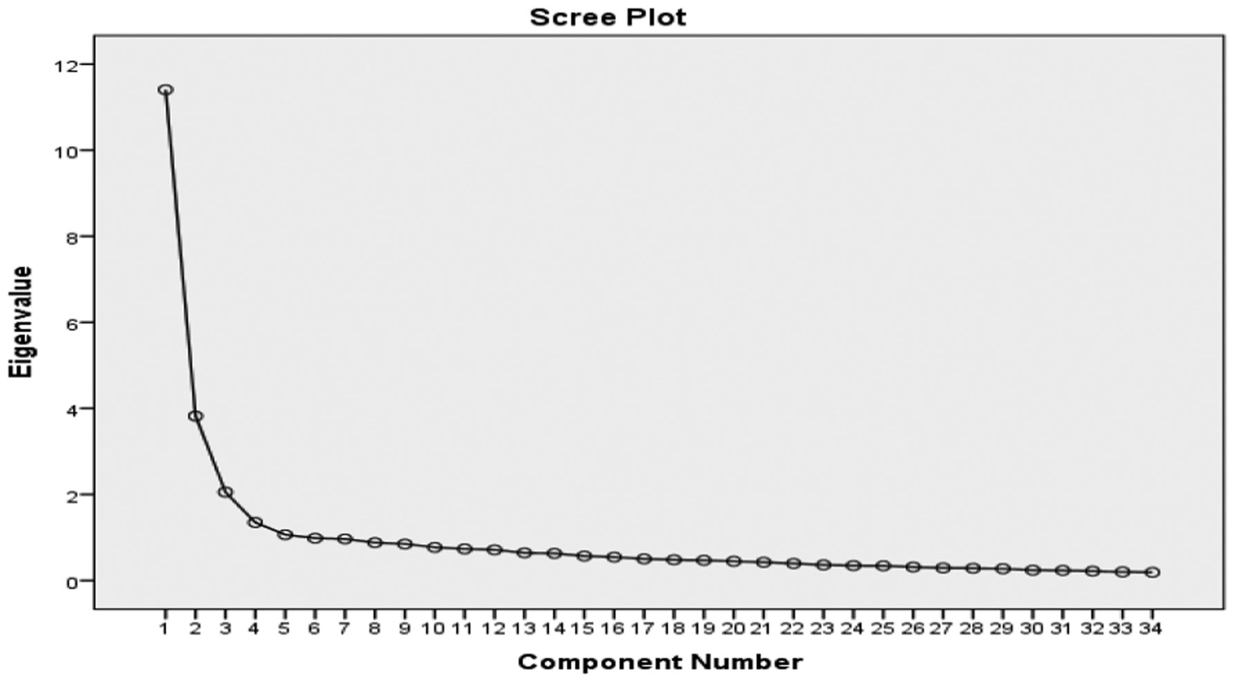
Social support has an important impact on the well-being of the elderly. Some studies have shown that perceived social support is more important than received social support. Perceived social support has different definitions across different age groups and cultures. So, this sequential exploratory mixed-method study was designed to develop and validate a perceived social support scale for community-dwelling elderly. In the qualitative phase, the perspectives of the elderly on perceived social support were defined through directed content analysis. Then, an extensive item pool was designed based on the elderly's perception and review of the literature. In the quantitative phase, the validity (content, face, and construct) and reliability (internal consistency, stability) of the newly developed scale was assessed using the sampling of five hundred elderly. The final scale consists of 34 items with domains of “emotional support”, “practical support”, “spiritual support”, “negative interactions” and “satisfaction with support received” that explained 58% of the total variance of the scale. The internal consistency varied from Cronbach's α = 0.70 to 0.87 for the subscales and as 0.92 for the whole scale. The study showed that the scale as a valid and reliable instrument can be used for the proper measurement of perceived social support among the elderly.

| [1] |
Antonucci TC, Ajrouch KJ, Birditt KS (2013) The Convoy Model: Explaining Social Relations From a Multidisciplinary Perspective. Gerontologist 54: 82-92. doi: 10.1093/geront/gnt118

|
| [2] |
Cheng C (2017) Anticipated support from children and later-life health in the United States and China. Soc Sci Med 179: 201-209. doi: 10.1016/j.socscimed.2017.03.007
|
| [3] |
Guo M, Li S, Liu J, et al. (2015) Family Relations, Social Connections, and Mental Health Among Latino and Asian Older Adults. Res Aging 37: 123-147. doi: 10.1177/0164027514523298
|
| [4] | Rezaee N, Ghajeh M (2009) Social Support among Nurses at Iran University of Medical Sciences. Hayat 14: 91-100. |
| [5] |
Cyranowski JM, Zill N, Bode R, et al. (2013) Assessing social support, companionship, and distress: National Institute of Health (NIH) Toolbox Adult Social Relationship Scales. Health Psychol 32: 293-301. doi: 10.1037/a0028586
|
| [6] |
Fiori KL, Denckla CA (2012) Social Support and Mental Health in Middle-Aged Men and Women:A Multidimensional Approach. J Aging Health 24: 407-438. doi: 10.1177/0898264311425087
|
| [7] |
Ahmed-Mohamed K, Fernandez-Mayoralas G, Rojo-Perez F, et al. (2013) Perceived Social Support of Older Adults in Spain. Appl Res Qual Life 8: 183-200. doi: 10.1007/s11482-012-9184-8
|
| [8] |
Gottlieb BH, Bergen AE (2010) Social support concepts and measures. J Psychosom Res 69: 511-520. doi: 10.1016/j.jpsychores.2009.10.001
|
| [9] |
Lubben J, Blozik E, Gillmann G, et al. (2006) Performance of an Abbreviated Version of the Lubben Social Network Scale Among Three European Community-Dwelling Older Adult Populations. Gerontologist 46: 503-513. doi: 10.1093/geront/46.4.503
|
| [10] |
Farokhnezhad Afshar P, Foroughan M, Vedadhir A, et al. (2017) Psychometric properties of the Persian version of Social Adaptation Self-evaluation Scale in community-dwelling older adults. Clini Interventions Aging 12: 579-584. doi: 10.2147/CIA.S129407
|
| [11] | Chen T, Ding Y, Spagnoletti P (2012) The role of social support network in e-health services for elderly persons Roma: IRIS—Institutional Research Information System, 1-12. |
| [12] |
Rodrigues MMS, De Jong Gierveld J, Buz J (2012) Loneliness and the exchange of social support among older adults in Spain and the Netherlands. Ageing Soc 34: 330-354. doi: 10.1017/S0144686X12000839
|
| [13] | Hosseinian M, Adib-Hajbaghery M, Amirkhosravi N (2013) An evaluation of social support and its influencing factors in the elderly of Bandar Abbas in 2013–2014. Life Sci J 10: 703-709. |
| [14] |
Abolfathi Momtaz Y, Ibrahim R, Hamid TA (2014) The impact of giving support to others on older adults' perceived health status. Psychogeriatrics 14: 31-37. doi: 10.1111/psyg.12036
|
| [15] | Grove SK, Burns N, Gray J (2012) The practice of nursing research: Appraisal, synthesis, and generation of evidence Elsevier Health Sciences. |
| [16] |
Elo S, Kyngäs H (2008) The qualitative content analysis process. J Adv Nurs 62: 107-115. doi: 10.1111/j.1365-2648.2007.04569.x
|
| [17] | Speziale HS, Streubert HJ, Carpenter DR (2011) Qualitative research in nursing: Advancing the humanistic imperative Lippincott Williams & Wilkins. |
| [18] | DiIorio CK (2006) Measurement in health behavior: methods for research and evaluation John Wiley & Sons. |
| [19] |
Krumpal I (2013) Determinants of social desirability bias in sensitive surveys: a literature review. Qual Quant 47: 2025-2047. doi: 10.1007/s11135-011-9640-9
|
| [20] |
Newman I, Lim J, Pineda F (2013) Content Validity Using a Mixed Methods Approach:Its Application and Development Through the Use of a Table of Specifications Methodology. J Mixed Methods Res 7: 243-260. doi: 10.1177/1558689813476922
|
| [21] | Polit D, Beck C (2012) Essentials of nursing research. Ethics 23: 145-160. |
| [22] |
Ayre C, Scally AJ (2014) Critical Values for Lawshe's Content Validity Ratio. Meas Eval Couns Dev 47: 79-86. doi: 10.1177/0748175613513808
|
| [23] |
Rust J, Golombok S (2014) Modern psychometrics: The science of psychological assessment Routledge. doi: 10.4324/9781315787527
|
| [24] | Brinkman WP (2009) Design of a questionnaire instrument. Handbook of Mobile Technology Research Methods NY: Nova Science Publisher, 31-57. |
| [25] |
Lacasse Y, Godbout C, Sériès F (2002) Health-related quality of life in obstructive sleep apnoea. Eur Respir J 19: 499-503. doi: 10.1183/09031936.02.00216902
|
| [26] | Corbin J, Strauss AL, Strauss A (2015) Basics of qualitative research Sage. |
| [27] | Munro BH (2005) Statistical methods for health care research Lippincott Williams & Wilkins. |
| [28] | Williams B, Onsman A, Brown T (2010) Exploratory factor analysis: A five-step guide for novices. Australas J Paramedicine 8. |
| [29] |
Kong F, Zhao J, You X (2012) Social support mediates the impact of emotional intelligence on mental distress and life satisfaction in Chinese young adults. Pers Individ Differ 53: 513-517. doi: 10.1016/j.paid.2012.04.021
|
| [30] |
Puustinen PJ, Koponen H, Kautiainen H, et al. (2011) Psychological distress measured by the GHQ-12 and mortality: A prospective population-based study. Scand J Public Health 39: 577-581. doi: 10.1177/1403494811414244
|
| [31] |
Montazeri A, Harirchi AM, Shariati M, et al. (2003) The 12-item General Health Questionnaire (GHQ-12): translation and validation study of the Iranian version. Health Qual Life Outcomes 1: 66. doi: 10.1186/1477-7525-1-66
|
| [32] |
Costa-Santos C, Bernardes J, Ayres-de-Campos D, et al. (2011) The limits of agreement and the intraclass correlation coefficient may be inconsistent in the interpretation of agreement. J Clin Epidemiol 64: 264-269. doi: 10.1016/j.jclinepi.2009.11.010
|
| [33] |
Wu S, Crespi CM, Wong WK (2012) Comparison of methods for estimating the intraclass correlation coefficient for binary responses in cancer prevention cluster randomized trials. Contemp Clin Trials 33: 869-880. doi: 10.1016/j.cct.2012.05.004
|
| [34] |
Nazari S, Foroughan M, Shahboulaghi FM, et al. (2016) Perceived social support in Iranian older adults: A qualitative study. Educ Gerontol 42: 443-452. doi: 10.1080/03601277.2016.1139970
|
| [35] |
McHugh ML (2012) Interrater reliability: the kappa statistic. Biochem Med 22: 276-282. doi: 10.11613/BM.2012.031
|
| [36] |
Polit DF, Beck CT, Owen SV (2007) Is the CVI an acceptable indicator of content validity? Appraisal and recommendations. Res Nurs Health 30: 459-467. doi: 10.1002/nur.20199
|
| [37] |
Sherbourne CD, Stewart AL (1991) The MOS social support survey. Soc Sci Med 32: 705-714. doi: 10.1016/0277-9536(91)90150-B
|
| [38] | Sarafino EP, Smith TW (2014) Health psychology: Biopsychosocial interactions John Wiley & Sons. |
| [39] |
Sarason IG, Sarason BR (2009) Social support: Mapping the construct. J Soc Pers Relat 26: 113-120. doi: 10.1177/0265407509105526
|
| [40] |
Caetano SC, Silva CM, Vettore MV (2013) Gender differences in the association of perceived social support and social network with self-rated health status among older adults: a population-based study in Brazil. BMC Geriatr 13: 122. doi: 10.1186/1471-2318-13-122
|
| [41] |
Taylor RJ, Forsythe-Brown I, Taylor HO, et al. (2014) Patterns of Emotional Social Support and Negative Interactions among African American and Black Caribbean Extended Families. J Afr Am Stud 18: 147-163. doi: 10.1007/s12111-013-9258-1
|
| [42] |
Thoits PA (2011) Mechanisms Linking Social Ties and Support to Physical and Mental Health. J Health Soc Behav 52: 145-161. doi: 10.1177/0022146510395592
|
| [43] |
Harvey IS, Alexander K (2012) Perceived social support and preventive health behavioral outcomes among older women. J Cross Cult Gerontol 27: 275-290. doi: 10.1007/s10823-012-9172-3
|
| [44] | Ahmad K (2011) Older adults' social support and its effect on their everyday self-maintenance activities: findings from the household survey of urban Lahore-Pakistan. S Asian Stud 26: 37. |
| [45] |
Huxhold O, Miche M, Schüz B (2014) Benefits of Having Friends in Older Ages: Differential Effects of Informal Social Activities on Well-Being in Middle-Aged and Older Adults. J Gerontol B Psychol Sci Soc Sci 69: 366-375. doi: 10.1093/geronb/gbt029
|
| [46] |
Siedlecki KL, Salthouse TA, Oishi S, et al. (2014) The Relationship Between Social Support and Subjective Well-Being Across Age. Soc Indic Res 117: 561-576. doi: 10.1007/s11205-013-0361-4
|
| [47] |
de Jager Meezenbroek E, Garssen B, van den Berg M, et al. (2012) Measuring Spirituality as a Universal Human Experience: A Review of Spirituality Questionnaires. J Relig Health 51: 336-354. doi: 10.1007/s10943-010-9376-1
|
| [48] |
Rushing NC, Corsentino E, Hames JL, et al. (2013) The relationship of religious involvement indicators and social support to current and past suicidality among depressed older adults. Aging Ment Health 17: 366-374. doi: 10.1080/13607863.2012.738414
|
| [49] |
Cornwell EY, Waite LJ (2009) Social Disconnectedness, Perceived Isolation, and Health among Older Adults. J Health Soc Behav 50: 31-48. doi: 10.1177/002214650905000103
|
| [50] |
Nguyen AW, Chatters LM, Taylor RJ, et al. (2016) Social Support from Family and Friends and Subjective Well-Being of Older African Americans. J Happiness Stud 17: 959-979. doi: 10.1007/s10902-015-9626-8
|
| [51] |
Rook KS (2015) Social Networks in Later Life:Weighing Positive and Negative Effects on Health and Well-Being. Curr Dir Psychol Sci 24: 45-51. doi: 10.1177/0963721414551364
|
| [52] |
Bastani S (2007) Family comes first: Men's and women's personal networks in Tehran. Soc Networks 29: 357-374. doi: 10.1016/j.socnet.2007.01.004
|
| [53] | Izadi S, Khamehvar A, Aram SS, et al. (2013) Social Support and Quality of Life of Elderly People admitted to Rehabilitation Centers. J Mazandaran Univ Med Sci 23: 101-109. |
| [54] |
Farokhnezhad Afshar P, Foroughan M, Vedadhi AA, et al. (2017) Relationship Between Social Function and Social Well-Being in Older Adults. Iran Rehabil J 15: 135-140. doi: 10.18869/nrip.irj.15.2.135
|
| [55] | (2016) Statistical Center of IranPopulation and Housing Censuses. Tehran: Statistical Center of Iran. |
| [56] |
Croezen S, Picavet HS, Haveman-Nies A, et al. (2012) Do positive or negative experiences of social support relate to current and future health? Results from the Doetinchem Cohort Study. BMC Public Health 12: 65. doi: 10.1186/1471-2458-12-65
|
| [57] |
Schwarzbach M, Luppa M, Forstmeier S, et al. (2014) Social relations and depression in late life—A systematic review. Int J Geriatr Psychiatry 29: 1-21. doi: 10.1002/gps.3971
|
 publichealth-07-01-007-s001.pdf publichealth-07-01-007-s001.pdf |
 |
Figures(1) / Tables(5)

Shima Nazari, Pouya Farokhnezhad Afshar, Leila Sadeghmoghadam, Alireza Namazi Shabestari, Akram Farhadi. Developing the perceived social support scale for older adults: A mixed-method study[J]. AIMS Public Health, 2020, 7(1): 66-80. doi: 10.3934/publichealth.2020007


 DownLoad: