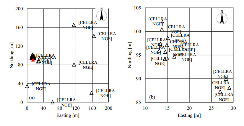
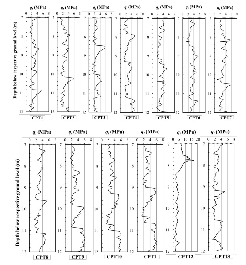
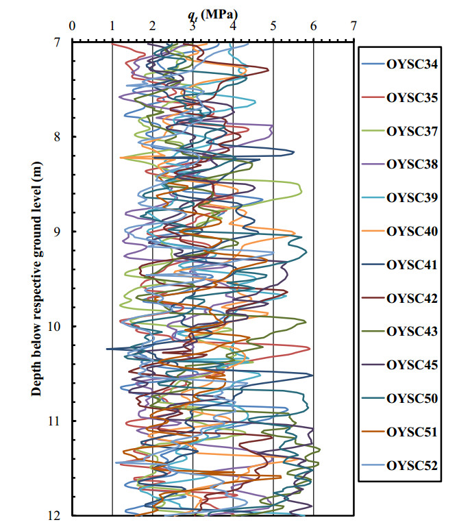
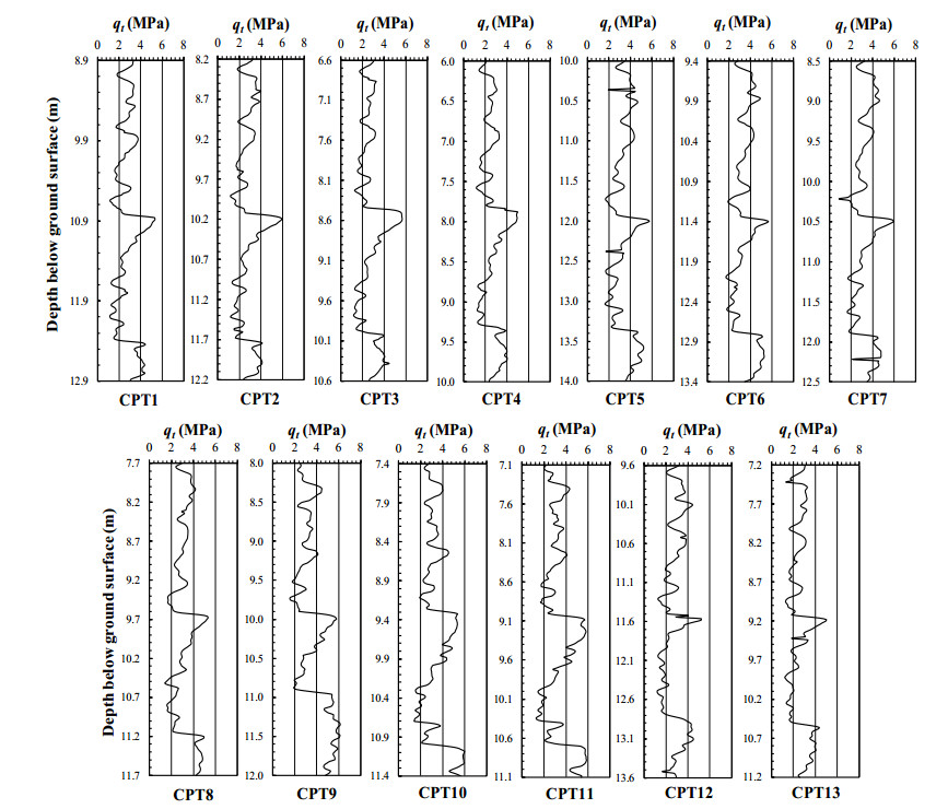
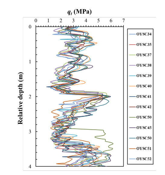
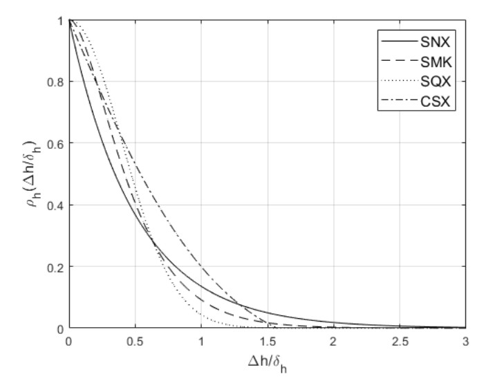
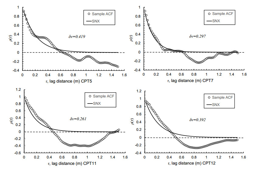
This paper presents a study of the spatial variability of the cone resistance in a medium dense sand deposit in Norway. Spatial variability studies have been done earlier for clay deposits, but there are few results available for sands. To bridge this gap and to compare the spatial variability of sand and clay, the in situ cone resistance measured with the piezocone at the Øysand benchmark site near Trondheim was studied. Corrected cone resistances qt derived from the measured cone resistance and pore pressure measurements were used to establish the autocorrelation structure of the Øysand deposit. The qt data were examined visually and conclusions were drawn on the data that should be analyzed. A depth interval of 7 to 12 m was selected for spatial variability further analysis. The scale of fluctuation was identified. Several autocorrelation functions were considered, and the single exponential function was found to be the one offering the best autocorrelation. The spatial variability in the vertical and horizontal directions was analyzed statistically, using three different approaches, the auto-correlation fitting, maximum likelihood estimation and simplified Vanmarcke method. The results indicate short autocorrelation distances of 3 m or less in the horizontal direction, suggesting a very variable sand at the Øysand site. These horizontal autocorrelation distances are much shorter than those obtained for clays. In the vertical direction the scale of fluctuation was less than one meter, as obtained for other soils.
Citation: Zhongqiang Liu, Åse Marit Wist Amdal, Jean-Sébastien L'Heureux, Suzanne Lacasse, Farrokh Nadim, Xin Xie. Spatial variability of medium dense sand deposit[J]. AIMS Geosciences, 2020, 6(1): 6-30. doi: 10.3934/geosci.2020002
This paper presents a study of the spatial variability of the cone resistance in a medium dense sand deposit in Norway. Spatial variability studies have been done earlier for clay deposits, but there are few results available for sands. To bridge this gap and to compare the spatial variability of sand and clay, the in situ cone resistance measured with the piezocone at the Øysand benchmark site near Trondheim was studied. Corrected cone resistances qt derived from the measured cone resistance and pore pressure measurements were used to establish the autocorrelation structure of the Øysand deposit. The qt data were examined visually and conclusions were drawn on the data that should be analyzed. A depth interval of 7 to 12 m was selected for spatial variability further analysis. The scale of fluctuation was identified. Several autocorrelation functions were considered, and the single exponential function was found to be the one offering the best autocorrelation. The spatial variability in the vertical and horizontal directions was analyzed statistically, using three different approaches, the auto-correlation fitting, maximum likelihood estimation and simplified Vanmarcke method. The results indicate short autocorrelation distances of 3 m or less in the horizontal direction, suggesting a very variable sand at the Øysand site. These horizontal autocorrelation distances are much shorter than those obtained for clays. In the vertical direction the scale of fluctuation was less than one meter, as obtained for other soils.

| [1] | Lacasse S, Nadim F (1996) Uncertainties in characterising soil properties. Uncertainty in the geologic environment: From theory to practice, ASCE, 49-75. |
| [2] |
Fenton GA (1999) Estimation for stochastic soil models. J Geotech Geoenviron Eng 125: 470-485. doi: 10.1061/(ASCE)1090-0241(1999)125:6(470)

|
| [3] | Liu Z, Lacasse S, Nadim F, et al. (2015) Accounting for the spatial variability of soil properties in the reliability−based design of offshore piles. Frontiers in Offshore Geotechnics Ⅲ: Proceedings of the 3rd Int. Symp. Frontiers in Offshore Geotechnics (ISFOG 2015). Taylor & Francis Books Ltd, 1375-1380. |
| [4] |
Ching J, Phoon KK, Sung SP (2017) Worst case scale of fluctuation in basal heave analysis involving spatially variable clays. Struct Saf 68: 28-42. doi: 10.1016/j.strusafe.2017.05.008
|
| [5] |
Phoon KK, Kulhawy FH (1999) Characterization of geotechnical variability. Can Geotech J 36: 612-624. doi: 10.1139/t99-038
|
| [6] |
Cheon JY, Gilbert RB (2014) Modeling spatial variability in offshore geotechnical properties for reliability—based foundation design. Struct Saf 49: 18-26. doi: 10.1016/j.strusafe.2013.07.008
|
| [7] |
Stuedlein AW, Kramer SL, Arduino P, et al. (2012) Geotechnical characterization and random field modeling of desiccated clay. J Geotech Geoenviron Eng 138: 1301-1313. doi: 10.1061/(ASCE)GT.1943-5606.0000723
|
| [8] |
Xiao T, Li DQ, Cao ZJ, et al. (2018) CPT-based probabilistic characterization of three−dimensional spatial variability using MLE. J Geotech Geoenviron Eng 144: 04018023. doi: 10.1061/(ASCE)GT.1943-5606.0001875
|
| [9] | L'Heureux JS, Lunne T, Lacasse S, et al. (2017) Norway's National GeoTest Site Research Infrastructure (NGTS). Unearth the Future, Connect beyond. Proc. 19th Int. Conf. Soil Mechanics and Geotechnical Engineering Seoul. |
| [10] |
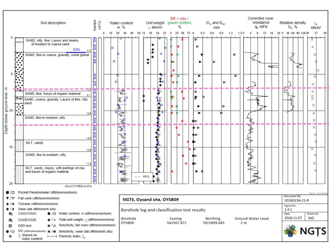
Quinteros S, Gundersen A, L'Heureux JS, et al. (2019) Øysand research site: Geotechnical characterization of deltaic sandy-silty soils. AIMS Geosci 5: 750-783. doi: 10.3934/geosci.2019.4.750
|
| [11] | Gundersen A, Quinteros S, L'Heureux JS, et al. (2018) Soil classification of NGTS sand site (Øysand, Norway) based on CPTU, DMT and laboratory results. Cone Penetration Testing 2018: Proceedings of the 4th Int. Symp. Cone Penetration Testing (CPT'18), 21-22 June, 2018, Delft, The Netherlands: CRC Press, 323. |
| [12] |
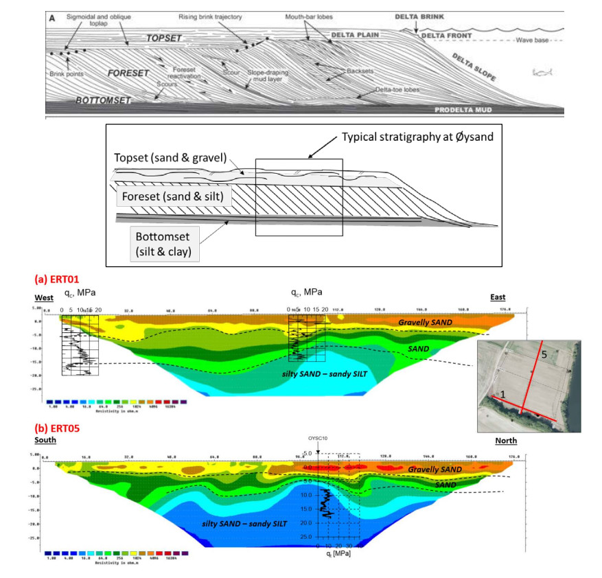
Gobo K, Ghinassi M, Nemec W (2015) Gilbert−type deltas recording short-term base-level changes: Delta-brink morphodynamics and related foreset facies. Sedimentology 62: 1923-1948. doi: 10.1111/sed.12212
|
| [13] |
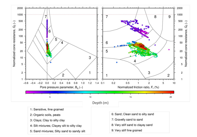
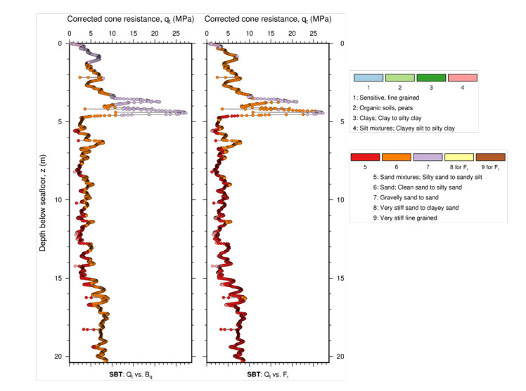
Robertson PK (1990) Soil classification using the cone penetration test. Can Geotech J 27: 151-158. doi: 10.1139/t90-014
|
| [14] | Lunne T, Powell JJM, Robertson PK (2002) Cone penetration testing in geotechnical practice. CRC Press, 312. |
| [15] | NGI (2017) Norwegian GeoTest Sites (NGTS). Factual report—Øysand Research site. Internal Report 20160154−24 Norwegian Geotechnical Institute (NGI) |
| [16] | NGI (2018) Norwegian Geo Test Sites (NGTS). Impact of cone penetrometer type on measured CPTU parameters at four NGTS sites. Silt, soft clay, sand and quick clay. Internal Report 20160154−30 Norwegian Geotechnical Institute (NGI). |
| [17] | Nadim F (1988) Geotechnical site description using stochastic interpolation. 10th Nordiske Geoteknikermøte, Oslo, Norway, 158-161. |
| [18] | Baecher GB, Christian JT (2003) Reliability and statistics in geotechnical engineering. John Wiley & Sons, 605. |
| [19] |
Vanmarcke EH (1977) Probabilistic modeling of soil profiles. J Geotech Eng Div 103: 1227-1246. doi: 10.1061/AJGEB6.0000517
|
| [20] | Nadim F (2015) Accounting for uncertainty and variability in geotechnical characterization of offshore sites. Proc of the 5th Int. Symp. Geotechnical Safety and Risk, 23-35. |
| [21] | Jaksa MB, Kaggwa WS, Brooker PI (1999) Experimental evaluation of the scale of fluctuation of a stiff clay. Proc 8th Int. Conf. Application of Statistics and Probability: Sydney, AA Balkema, Rotterdam, 415-422. |
| [22] |
Uzielli M, Vannucchi G, Phoon KK (2005) Random field characterisation of stress−nomalised cone penetration testing parameters. Geotechnique 55: 3-20. doi: 10.1680/geot.2005.55.1.3
|
| [23] | Hoeg K, Tang W (1977) Probabilistic considerations in the foundation engineering for offshore structures. Proc. Int. Conf. Structural Safety and Reliability 2. Munich, 267-296. |
| [24] | Tang WH (1979) Probabilistic evaluation of penetration resistances. J Geotech Geoenviron Eng 105: 1173−1191. |
| [25] | Keaveny JM, Nadim F, Lacasse S (1989) Autocorrelation functions for offshore geotechnical data. Structural Safety and Reliability: ASCE, 263-270. |
| [26] | Lacasse S, de Lamballerie JY (1995) Statistical treatment of CPT data. Proc. Int. Symp. on Cone Penetration Testing, 4-5. |
| [27] | Alonso EE, Krizek RJ (1975) Stochastic formulation of soil properties. In Proc., 2nd Int. Conf. Applications of Statistics & Probability in Soil and Structural Engineering, Aachen, 9-32. |
| [28] | Baecher G (1985) Geotechnical error analysis. Transp Res Rec, 23-31. |
| [29] | Campanella RG, Wickremesinghe DS, Robertson PK (1987) Statistical treatment of cone penetrometer test data. Proc. 5th Int. Conf. Application of Statistics and Probability, 1011-1019. |
| [30] | Kulatilake PHS, Ghosh A (1988) An investigation into accuracy of spatial variation estimation using static cone penetrometer data. Proc. 1st Int. Conf. Penetration Testing, Orlando, Fla, 815-821. |
| [31] |
Chiasson P, Lafleur J, Soulié M, et al. (1995) Characterizing spatial variability of a clay by geostatistics. Can Geotech J 32: 1-10. doi: 10.1139/t95-001
|
| [32] | DeGroot DJ (1996) Analyzing spatial variability of in situ soil properties. Uncertainty in the geologic environment: From theory to practice, ASCE, 210-238. |
| [33] | Hegazy YA, Mayne PW, Rouhani S (1996) Geostatistical assessment of spatial variability in piezocone tests. Uncertainty in the geologic environment: from theory to practice, ASCE, 254-268. |
| [34] |
Cafaro F, Cherubini C (2002) Large sample spacing in evaluation of vertical strength variability of clayey soil. J Geotech Geoenviron Eng 128: 558-568. doi: 10.1061/(ASCE)1090-0241(2002)128:7(558)
|
| [35] | Gauer P, Lunne T (2002) Statistical Analyses of CPTU data from Onsøy. Internal Report 20001099−2 Norwegian Geotechnical Institute. |
| [36] |
Kulatilake PHSW, Um JG (2003) Spatial variation of cone tip resistance for the clay site at Texas A & M University. Geotech Geol Eng 21: 149-165. doi: 10.1023/A:1023526614301
|
| [37] |
Elkateb T, Chalaturnyk R, Robertson PK (2003) An overview of soil heterogeneity: quantification and implications on geotechnical field problems. Can Geotech J 40: 1-15. doi: 10.1139/t02-090
|
| [38] | Uzielli M, Lacasse S, Nadim F, et al. (2006) Soil variability analysis for geotechnical practice. In Tan TS, Phoon KK, Hight DW, et al., Characterization and engineering properties of natural soils 3: 1653-1752. |
| [39] |
Liu CN, Chen CH (2006) Mapping liquefaction potential considering spatial correlations of CPT measurements. J Geotech Geoenviron Eng 132: 1178-1187. doi: 10.1061/(ASCE)1090-0241(2006)132:9(1178)
|
| [40] | Li LJH, Uzielli M, Cassidy M (2015) Uncertainty−based characterization of Piezocone and T−bar data for the Laminaria offshore site. Frontiers in Offshore Geotechnics Ⅲ: Proc. 3rd Int. Symp. Frontiers in Offshore Geotechnics (ISFOG 2015), Taylor & Francis Books Ltd, 1381-1386. |
| [41] |
Ching J, Wu TJ, Stuedlein AW, et al. (2018) Estimating horizontal scale of fluctuation with limited CPT soundings. Geosci Front 9: 1597-1608. doi: 10.1016/j.gsf.2017.11.008
|
| [42] |
DeGroot DJ, Baecher GB (1993) Estimating autocovariance of in−situ soil properties. J Geotech Eng 119: 147-166. doi: 10.1061/(ASCE)0733-9410(1993)119:1(147)
|
| [43] | Hammer HB (2019) Accuracy of CPTUs in deltaic sediments and the effect of cone penetrometer type. Project thesis—TBA4510. Norwegian University of Science and Technology. Trondheim, Norway. |
| [44] | Nie X, Huang H, Liu Z, et al. (2015) Scale of fluctuation for geotechnical probabilistic analysis. In Schweckendiek T, van Tol AF, Pereboom D, et al., Proc. ISGSR2015: Geotechnical Safety and Risk V, IOS Press, 816-821. |
Figures(13) / Tables(8)

Zhongqiang Liu, Åse Marit Wist Amdal, Jean-Sébastien L'Heureux, Suzanne Lacasse, Farrokh Nadim, Xin Xie. Spatial variability of medium dense sand deposit[J]. AIMS Geosciences, 2020, 6(1): 6-30. doi: 10.3934/geosci.2020002


 DownLoad: