Loading [MathJax]/jax/output/SVG/jax.js
Research article Special Issues

Influence of dirt and coating deterioration on the aging of solar reflectance of high-reflectance paint

  • Received: 29 July 2019 Accepted: 10 September 2019 Published: 22 October 2019
  • Cool-roof coatings have received considerable attention worldwide as a solution for the “heat island” effect in urban areas. The solar reflectance of roofs coated with high-reflectance paint is reduced by dirt. We continuously measured the solar reflectance of a roof coated with high-reflectance paint with and without a self-cleaning function for more than two years. The solar reflectance of self-cleaning paint decreased by 0.5% per month over two years, due to the effect of dirt. The solar reflectance of conventional paint decreased by 4% per month over four months after coating and then reached a value similar to that for the self-cleaning paint for two years due to deterioration. With a slight decrease in solar reflectance, the self-cleaning function is effective in mitigating the heat island effect and obtaining continuous energy-savings. We applied the alkyl silicate system as self-cleaning for high-reflectance paint, the solar reflectance was measured continuously at 1 minute intervals, and the actual state of the fluctuation in reflectance over the short and long terms was analyzed with the influence of the altitude of the sun. The deterioration of the coating was also investigated by gloss retention and chalking test.

    Citation: Taizo Aoyama, Takeshi Sonoda, Hideki Takebayashi. Influence of dirt and coating deterioration on the aging of solar reflectance of high-reflectance paint[J]. AIMS Materials Science, 2019, 6(6): 997-1009. doi: 10.3934/matersci.2019.6.997

    Related Papers:

    [1] Elias Maciel, Inocencio Ortiz, Christian E. Schaerer . A Herglotz-based integrator for nonholonomic mechanical systems. Journal of Geometric Mechanics, 2023, 15(1): 287-318. doi: 10.3934/jgm.2023012
    [2] Xavier Rivas, Daniel Torres . Lagrangian–Hamiltonian formalism for cocontact systems. Journal of Geometric Mechanics, 2023, 15(1): 1-26. doi: 10.3934/jgm.2023001
    [3] Jordi Gaset, Arnau Mas . A variational derivation of the field equations of an action-dependent Einstein-Hilbert Lagrangian. Journal of Geometric Mechanics, 2023, 15(1): 357-374. doi: 10.3934/jgm.2023014
    [4] Alexander Pigazzini, Cenap Özel, Saeid Jafari, Richard Pincak, Andrew DeBenedictis . A family of special case sequential warped-product manifolds. Journal of Geometric Mechanics, 2023, 15(1): 116-127. doi: 10.3934/jgm.2023006
    [5] Marcin Zając . The dressing field method in gauge theories - geometric approach. Journal of Geometric Mechanics, 2023, 15(1): 128-146. doi: 10.3934/jgm.2023007
    [6] Robert I McLachlan, Christian Offen . Backward error analysis for conjugate symplectic methods. Journal of Geometric Mechanics, 2023, 15(1): 98-115. doi: 10.3934/jgm.2023005
    [7] Álvaro Rodríguez Abella, Melvin Leok . Discrete Dirac reduction of implicit Lagrangian systems with abelian symmetry groups. Journal of Geometric Mechanics, 2023, 15(1): 319-356. doi: 10.3934/jgm.2023013
    [8] Markus Schlarb . A multi-parameter family of metrics on stiefel manifolds and applications. Journal of Geometric Mechanics, 2023, 15(1): 147-187. doi: 10.3934/jgm.2023008
    [9] Valentin Duruisseaux, Melvin Leok . Time-adaptive Lagrangian variational integrators for accelerated optimization. Journal of Geometric Mechanics, 2023, 15(1): 224-255. doi: 10.3934/jgm.2023010
    [10] Francesco Bonechi, Jian Qiu, Marco Tarlini . Generalised Kähler structure on CP2 and elliptic functions. Journal of Geometric Mechanics, 2023, 15(1): 188-223. doi: 10.3934/jgm.2023009
  • Cool-roof coatings have received considerable attention worldwide as a solution for the “heat island” effect in urban areas. The solar reflectance of roofs coated with high-reflectance paint is reduced by dirt. We continuously measured the solar reflectance of a roof coated with high-reflectance paint with and without a self-cleaning function for more than two years. The solar reflectance of self-cleaning paint decreased by 0.5% per month over two years, due to the effect of dirt. The solar reflectance of conventional paint decreased by 4% per month over four months after coating and then reached a value similar to that for the self-cleaning paint for two years due to deterioration. With a slight decrease in solar reflectance, the self-cleaning function is effective in mitigating the heat island effect and obtaining continuous energy-savings. We applied the alkyl silicate system as self-cleaning for high-reflectance paint, the solar reflectance was measured continuously at 1 minute intervals, and the actual state of the fluctuation in reflectance over the short and long terms was analyzed with the influence of the altitude of the sun. The deterioration of the coating was also investigated by gloss retention and chalking test.


    In the last few decades, more and more scholars have studied fractional-order neural networks (FONNs) due to their powerful functions [1,2]. FONNs have been accurately applied to image processing, biological systems and so on [3,4,5,6] because of their powerful computing power and information storage capabilities. In the past, scholars have studied many types of neural network (NN) models. For example, bidirectional associative memory neural networks (BAMNNs) [7], recurrent NNs [8], Hopfield NNs [9], Cohen-Grossberg NNs [10], and fuzzy neural networks (FNNs) [11]. With the development of fuzzy mathematics, Yang et al. proposed fuzzy logic (fuzzy OR and fuzzy AND) into cellular NNs and established FNNs. Moreover, when dealing with some practical problems, it is inevitable to encounter approximation, uncertainty, and fuzziness. Fuzzy logic is considered to be a promising tool to deal with these phenomena. Therefore, the dynamical behaviors of FNNs have attracted extensive research and obtained abundant achievements [12,13,14,15].

    The CVNNs are extended from real-valued NNs (RVNNs). In CVNNs, the relevant variables in CVNNs belong to the complex field. In addition, CVNNs can also address issues that can not be addressed by RVNNs, such as machine learning [16] and filtering [17]. In recent years, the dynamic behavior of complex valued neural networks has been a hot topic of research for scholars. In [16], Nitta derived some results of an analysis on the decision boundaries of CVNNs. In [17], the author studied an extension of the RBFN for complex-valued signals. In [18], Li et al. obtained some synchronization results of CVNNs with time delay. Overall, CVNNs outperform real-valued neural networks in terms of performance, as they can directly process two-dimensional data.

    Time delays are inescapable in neural systems due to the limited propagation velocity between different neurons. Time delay has been extensively studied by previous researchers, such as general time delay [19], leakage delays [20], proportional delays [21], discrete delays [22], time-varying delays [23], and distributed delays [24]. In addition, the size and length of axonal connections between neurons in NNs can cause time delays, so scholars have introduced distributed delays in NNs. For example, Si et al. [25] considered a fractional NN with distributed and discrete time delays. It not only embodies the heredity and memory characteristics of neural networks but also reflects the unevenness of delay in the process of information transmission due to the addition of distributed time delays. Therefore, more and more scholars have added distributed delays to the NNs and have made some new discoveries [26,27]. On the other hand, due to the presence of external perturbations in the model, the actual values of the parameters in the NNs cannot be acquired, which may lead to parameter uncertainties. Parameter uncertainty has also affected the performance of NNs. Consequently, scholars are also closely studying the NNs model of parameter uncertainty [28,29].

    The synchronization control of dynamical systems has always been the main aspect of dynamical behavior analysis, and the synchronization of NNs has become a research hotspot. In recent years, scholars have studied some important synchronization behaviors, such as complete synchronization (CS) [30], global asymptotic synchronization [31], quasi synchronization [32], finite time synchronization [33], projective synchronization (PS) [34], and Mittag-Leffler synchronization (MLS) [35]. In various synchronizations, PS is one of the most interesting, being characterized by the fact that the drive-response systems can reach synchronization according to a scaling factor. Meanwhile, the CS can be regarded as a PS with a scale factor of 1. Although PS has its advantages, MLS also has its unique features. Unlike CS, MLS can achieve synchronization at a faster speed. As a result, some scholars have combined the projective synchronization and ML synchronization to study MLPS [36,37]. However, there are few papers on MLPS of FOFNNs. Based on the above discussion, the innovative points of this article are as follows:

    According to the FNNs model, parameter uncertainty and distributed delays are added, and the influence of time-varying delay, distributed delay, and uncertainty on the global MLPS of FOFCVNNs is further considered in this paper.

    The algebraic criterion for MLPS was obtained by applying the complex valued direct method. Direct methods and algebraic inequalities greatly reduce computational complexity.

    The design of nonlinear hybrid controllers and adaptive hybrid controllers greatly reduces control costs.

    Notations: In this article, C refers to the set of complex numbers, where O=OR+iOIC and OR,OIR, i represents imaginary units, Cn can describe a set of n-dimensional complex vectors, ¯Oψ refers to the conjugate of Oψ. |Oψ|=Oψ¯Oψ indicating the module of Oψ. For O=(O1,O2,,On)TCn,||O||=(nψ=1|Oψ|2)12 denotes the norm of O.

    In this section, we provide the definitions, lemmas, assumptions, and model details required for this article.

    Definition 2.1. [38] The Caputo fractional derivative with 0<Υ<1 of function O(t) is defined as

    ct0DαtO(t)=1Γ(1α)tt0O(s)(ts)αds.

    Definition 2.2. [38] The one-parameter ML function is described as

    EΥ(p)=δ=0pδΓ(δΥ+1).

    Lemma 2.1. [39] Make Qψ,OψC(w,ψ=1,2,,n,), then the fuzzy operators in the system satisfy

    |nψ=1μwψfψ(Qψ)nψ=1μwψfψ(Oψ)|nψ=1|μwψ||fψ(Qψ)fψ(Oψ)|,|nψ=1υwψfψ(Qψ)nψ=1υwψfψ(Oψ)|nψ=1|υwψ||fψ(Qψ)fψ(Oψ)|.

    Lemma 2.2. [40] If the function ϑ(t)C is differentiable, then it has

    Ct0Dαt(¯ϑ(t)ϑ(t))ϑ(t)Ct0Dαtϑ(t)+(Ct0Dαt¯ϑ(t))ϑ(t).

    Lemma 2.3. [41] Let ˆξ1,ˆξ2C, then the following condition:

    ¯ˆξ1ˆξ2+¯ˆξ2ˆξ1χ¯ˆξ1ˆξ1+1χ¯ˆξ2ˆξ2

    holds for any positive constant χ>0.

    Lemma 2.4. [42] If the function ς(t) is nondecreasing and differentiable on [t0,], the following inequality holds:

    ct0Dαt(ς(t)ȷ)22(ς(t)ȷ)ct0Dαt(ς(t)), 0<α<1,

    where constant ȷ is arbitrary.

    Lemma 2.5. [43] Suppose that function (t) is continuous and satisfies

    ct0Dαtˆ(t)γˆ(t),

    where 0<α<1, γR, the below inequality can be obtained:

    ˆ(t)ˆ(t0)Eα[γ(tt0)α].

    Next, a FOFCVNNS model with distributed and time-varying delays with uncertain coefficients is considered as the driving system:

    Ct0DαtOw(t)=awOw(t)+nψ=1(mwψ+Δmwψ(t))fψ(Oψ(tτ(t)))+nψ=1μwψ+0bwψ(t)fψ(Oψ(t))dt+nψ=1υwψ+0cwψ(t)fψ(Oψ(t))dt+Iw(t), (2.1)

    where 0<α<1; O(t)=((O1(t),...,On(t)); Ow(t),w=1,2,...,n is the state vector; awR denotes the self-feedback coefficient; mwψC stands for a feedback template element; mwψC refers to uncertain parameters; μwψC and υwψC are the elements of fuzzy feedback MIN and MAX templates; and indicate that the fuzzy OR and fuzzy AND operations; τ(t) indicates delay; Iw(t) denotes external input; and fψ() is the neuron activation function.

    Correspondingly, we define the response system as follows:

    Ct0DαtQw(t)=awQw(t)+nψ=1(mwψ+Δmwψ(t))fψ(Qψ(tτ(t)))+nψ=1μwψ+0bwψ(t)fψ(Qψ(t))dt+nψ=1υwψ+0cwψ(t)fψ(Qψ(t))dt+Iw(t)+Uw(t), (2.2)

    where Uw(t)C stands for controller. In the following formula, Ct0Dαt is abbreviated as Dα.

    Defining the error as kw(t)=Qw(t)SOw(t), where S is the projective coefficient. Therefore, we have

    Dαkw(t)=awkw(t)+nψ=1(mwψ+Δmwψ(t))~fψkψ(tτ(t))+nψ=1(mwψ+Δmwψ(t))fψ(SOψ(tτ(t)))nψ=1S(mwψ+Δmwψ(t))fψ(Oψ(tτ(t)))+nψ=1μwψ+0bwψ(t)fψ~kψ(t)dt+nψ=1μwψ+0bwψ(t)fψ(SOψ(t))dtSnψ=1μwψ+0bwψ(t)fψ(Oψ(t))dt+nψ=1υwψ+0cwψ(t)fψ~kψ(t)dt+nψ=1υwψ+0cwψ(t)fψ(SOψ(t))dtSnψ=1υwψ+0cwp(t)fψ(Oψ(t))dt+(1S)Iw(t)+Uw(t), (2.3)

    where fψ~kψ(t)=fψ(Qψ(t))fψ(SOψ(t)).

    Assumption 2.1. O,QC and Lϖ>0, fϖ() satisfy

    |fϖ(O)fϖ(Q)|Lϖ|OQ|.

    Assumption 2.2. The nonnegative functions bwψ(t) and cwψ(t) are continuous, and satisfy

    (i)+0bwψ(t)dt=1,(ii)+0cwψ(t)dt=1.

    Assumption 2.3. The parameter perturbations mwψ(t) bounded, then it has

    |mwψ(t)|Mwψ,

    where Mwψ is all positive constants.

    Assumption 2.4. Based on the assumption for fuzzy OR and AND operations, the following inequalities hold:

    (i)[nψ=1μwψ+0bwψ(t)(fψ(Oψ)fψ(Qψ))dt][nψ=1¯μwψ+0bwψ(t)(fψ(Oψ)fψ(Qψ))dt]nψ=1δψ|μwψ|2(fψ(Oψ)fψ(Qψ))(¯fψ(Oψ)¯fψ(Qψ)),(ii)[nψ=1υwψ+0cwψ(t)(fψ(Oψ)fψ(Qψ))dt][nψ=1¯υwψ+0cwψ(t)(fψ(Oψfψ(Qψ))dt]nψ=1ηψ|υwψ|2(fψ(Oψ)fψ(Qψ))(¯fψ(Oψ)¯fψ(Qψ)),

    where δψ and ηψ are positive numbers.

    Definition 2.3. The constant vector O=(O1,,On)TCn and satisfy

    0=awOψ+nψ=1(mwψ+mwψ(t))fψ(Oψ)+nψ=1μwψ+0bwψ(t)fψ(Oψ)dt+nψ=1υwψ+0cwψ(t)fψ(Oψ)dt+Iw(t),

    whereupon, O is called the equilibrium point of (2.1).

    Definition 2.4. System (2.1) achieves ML stability if and only if O=(O1,,On)TCn is the equilibrium point, and satisfies the following condition:

    ||O(t)||[Ξ(O(t0))Eα(ρ(tt0)α)]η,

    where 0<α<1,ρ, η>0,Ξ(0)=0.

    Definition 2.5. If FOFCVNNS (2.1) and (2.2) meet the following equation:

    limtQw(t)SOw(t)=0,

    so we can say it has achieved projective synchronization, where SR is projective coefficient.

    In this part, we mainly investigate three theorems. According to the Banach contraction mapping principle, we can deduce the result of Theorem 3.1. Next, we construct a linear hybrid controller and an adaptive hybrid controller, and establish two MLPS criteria.

    Theorem 3.1. B is a Banach space. Let ||O||1=nψ=1|Oψ|. Under Assumptions 2.1–2.4, if the following equality holds:

    ρ=nw=1|mwψ|Lψ+|Mwψ|Lψ+|μwψ|Lψ+|υwψ|Lψaψ<1,w,ψ=1,2,3,...,n, (3.1)

    then FOFCVNNS (2.1) has a unique equilibrium point with O=(O1,,On)TCn.

    Proof. Let O=(~O1,~O2,,~On)=(a1O1,a2O2,,anOn)Rn, and construct a mapping φ:BB, φ(x)=(φ1(O),φ2(O),,φn(O)) and

    φψ(O)=nψ=1(mwψ+Δmwψ(t))fψ(~Oψaψ)+nψ=1μwψ+0bwψ(t)fψ(~Oψaψ)dt+nψ=1υwψ+0cwψ(t)fψ(~Oψaψ)dt+Iw,w,ψ=1,2,,n. (3.2)

    For two different points α=(α1,,αn),β=(β1,,βn), it has

    |φψ(α)φψ(β)||nψ=1(mwψ+Δmwψ(t))fψ(αψaψ)nψ=1(mwψ+Δmwψ(t))fψ(βψaψ)|+|nψ=1μwψ+0bwψ(t)fψ(αψaψ)dtnψ=1μwψ+0bwψ(t)fψ(βψaψ)dt|+|nψ=1υwψ+0cwψ(t)fψ(αψaψ)dtnψ=1υwψ+0cwψ(t)fψ(βψaψ)dt|nψ=1|mwψ+Δmwψ(t)||fj(αψaψ)fψ(βψaψ)|+|nψ=1μwψfψ(αψaψ)nψ=1μwψfψ(βψaψ)|+|nψ=1υwψfp(αψaψ)nψ=1υwψfψ(βψaψ)|. (3.3)

    According to Assumption 2.1, we get

    |φψ(α)φψ(β)|nψ=1|mwψ+Δmwψ(t)|Lψaψ|αψβψ|+nψ=1|μwψ|Lψaψ|αψβψ|+nψ=1|υwψ|Lψaψ|αψβψ|. (3.4)

    Next, we have

    ||φ(α)φ(β)||1=nψ=1|φψ(α)φψ(β)|nψ=1nψ=1|mwψ+Δmwψ(t)|Lψaψ|αψβψ|+nw=1nψ=1|μwψ|Lψaψ|αψβψ|+nw=1nψ=1|υwψ|Lψaψ|αψβψ|nψ=1(nψ=1|mwψ+Δmwψ(t)|Lψaψ+nψ=1|μwψ|Lψaψ+nw=1|υwψ|Lψaψ)|αψβψ|(nw=1|mwψ+Δmwψ(t)|Lψaψ+nw=1|μwψ|Lψaψ+nw=1|υwψ|Lψaψ)nψ=1|αψβψ|. (3.5)

    From Assumption 2.3, then it has

    ||φ(α)φ(β)||1(nw=1|mwψ|Lψ+|Mwψ|Lψ+|μwψ|Lp+|υwψ|Lψaψ)||αβ||1. (3.6)

    Finally, we obtain

    ||φ(α)φ(β)||1ρ||αβ||1, (3.7)

    where φ is obviously a contraction mapping. From Eq (3.2), there must exist a unique fixed point ~OCn, such that φ(~O)=~O.

    ~Oψ=nψ=1(mwψ+Δmwψ(t))fψ(~Oψaψ)+nψ=1μwψ+0bwψ(t)fψ(~Oψaψ)dt+nψ=1υwψ+0cwψ(t)fψ(~Oψaψ)dt+Iw. (3.8)

    Let Oψ=~Oψaψ, we have

    0=awOψ+nψ=1(mwψ+Δmwψ(t))fψ(Oψ)+nψ=1μwψ+0bwψ(t)fψ(Oψ)dt+nψ=1υwψ+0cwψ(t)fψ(Oψ)dt+Iw. (3.9)

    Consequently, Theorem 3.1 holds.

    Under the error system (2.3), we design a suitable hybrid controller

    uw(t)=u1w(t)+u2w(t). (3.10)
    u1w(t)={πkw(t)+λkw(t)¯kw(tτ(t))¯kw(t),kw(t)0,0,kw(t)=0. (3.11)
    u2w(t)=nψ=1(mwψ+Δmwψ(t))fψ(SOψ(tτ(t)))+nψ=1S(mwψ+Δmwψ(t))fψ(Oψ(tτ(t)))nψ=1μwψ+0bwψ(t)fψ(SOψ(t))dt+Snψ=1μwψ+0bwψ(t)fψ(Oψ(t))dtnψ=1υwψ+0cwψ(t)fψ(SOψ(t))dt+Snψ=1υwψ+0cwψ(t)fψ(Oψ(t))dt(1h)Iψ. (3.12)

    By substituting (3.10)–(3.12) into (2.3), it yields

    Dαkw(t)=awkw(t)+nψ=1(mwψ+Δmwψ(t))~fψkψ(tτ(t))+nψ=1μwψ+0bwψ(t)fψ~kψ(t)dt+nψ=1υwψ+0cwψ(t)fψ~kψ(t)dtπkw(t)+λkw(t)¯kw(tτ(t))¯kw(t). (3.13)

    Theorem 3.2. Based on the controller (3.10) and Assumptions 2.1–2.4, systems (2.1) and (2.2) can achieve MLPS if the following formula holds:

    ϖ1=min1wn{2awλ+2π4nnψ=1δw|μψw|2L2wnψ=1ηw|υψw|2L2w}>0,ϖ2=max1wn{λ+nψ=1(|mψw|2+|Mψw|2)L2w},ϖ1ϖ2Ω1>0,Ω1>1. (3.14)

    Proof. Picking the Lyapunov function as

    v1(t)=nw=1kw(t)¯kw(t). (3.15)

    By application about derivative v1(t), we derive

    Dαv1(t)=nw=1Dαkw(t)¯kw(t). (3.16)

    Following Lemma 2.2, it has

    Dαv1(t)nw=1kw(t)Dα¯kw(t)+nw=1¯kw(t)Dαkw(t). (3.17)

    Substituting Eq (3.13) to (3.17), we can get

    Dαv1(t)nw=1kw(t){aw¯kw(t)+nψ=1¯(mwψ+mwψ(t))¯~fψkψ(tτ(t))+nψ=1¯μwψ+0bwψ(t)fψ~kψ(t)dt+nψ=1¯υwψ+0cwψ(t)fψ~kψ(t)dtπ¯kw(t)+λ¯kw(t)¯kw(tτ(t))kw(t)}+nw=1¯kw(t){awkw(t)+nψ=1(mwp+Δmwψ(t))~fψkψ(tτ(t))+nψ=1μwψ+0bwψ(t)fψ~kψ(t)dt+nψ=1υwψ+0cwψ(t)fψ~kψ(t)dtπkw(t)+λkw(t)¯kw(tτ(t))¯kw(t)}. (3.18)

    Combining Lemma 2.3, one gets

    nw=1kw(t)λ¯kw(t)¯kw(tτ(t))kw(t)+nw=1¯kw(t)λkw(t)¯kw(tτ(t))¯kw(t)λnw=1(kw(t)¯kw(t)+kw(tτ(t))¯kw(tτ(t))). (3.19)

    Based on (3.19), we derive

    nw=1kw(t)(aw¯kw(t)π¯kw(t)+λ¯kw(t)¯kw(tτ(t))kw(t))+nw=1¯kw(t)(awkw(t)πkw(t)+λkw(t)¯kw(tτ(t))¯kw(t))nw=1[2awλ+2π]kw(t)¯kw(t)+λnw=1kw(tτ(t))¯kw(tτ(t)). (3.20)

    According to Assumptions 2.1 and 2.3, Lemma 2.3, we can get

    nw=1nψ=1[kw(t)¯mwψ¯~fψkψ(tτ(t))+kw(t)¯mwψ(t)¯~fψkψ(tτ(t))+¯kw(t)mwψ~fψkψ(tτ(t))+¯kw(t)mwψ(t)~fψkψ(tτ(t))]nw=1nψ=1[2kw(t)¯kw(t)+|mwψ|2~fψkψ(tτ(t))¯~fψkψ(tτ(t))+|mwψ(t)|2~fψkψ(tτ(t))¯~fψkψ(tτ(t))]nw=1nψ=12kw(t)¯kw(t)+nw=1nψ=1|mwψ|2L2ψkψ(tτ(t))¯kψ(tτ(t))+nw=1nψ=1|Mwψ|2L2ψkψ(tτ(t))¯kψ(tτ(t))nw=1nψ=12kw(t)¯kw(t)+nw=1nψ=1(|mwψ|2+|Mwψ|2)L2ψkψ(tτ(t))¯kψ(tτ(t)). (3.21)

    Based on Lemma 2.3, one has

    nw=1[kw(t)nψ=1¯μwψ+0bwψ(t)fψ~kψ(t)dt+¯kw(t)nψ=1μwψ+0bwψ(t)fψ~kψ(t)dt]nw=1[kw(t)¯kw(t)+nψ=1μwψ+0bwψ(t)fψ~kψ(t)dtnψ=1¯μwψ+0bwψ(t)fψ~kψ(t)dt]. (3.22)

    Combining Assumption 2.4 and Lemma 2.1, one obtains

    nw=1nψ=1μwψ+0bwψ(t)fψ~kψ(t)dtnψ=1¯μwψ+0bwψ(t)fψ~kψ(t)dtnw=1nψ=1δψ|μwψ|2L2ψkψ(t)¯kψ(t). (3.23)

    Substituting (3.23) into (3.22), it has

    nw=1[kw(t)nψ=1¯μwψ+0bwψ(t)fψ~kψ(t)dt+¯kw(t)nψ=1μwψ+0bwψ(t)fψ~kψ(t)dt]nw=1kw(t)¯kw(t)+nw=1nψ=1δψ|μwψ|2L2ψkψ(t)¯kψ(t). (3.24)

    Thus,

    nw=1[kw(t)nψ=1¯υwψ+0cwψ(t)fψ~kψ(t)dt+¯kw(t)nψ=1υwψ+0cwψ(t)fψ~kψ(t)dt]nw=1kw(t)¯kw(t)+nψ=1nψ=1ηψ|υwψ|2L2ψkψ(t)¯kψ(t). (3.25)

    Substituting (3.20)–(3.25) into (3.18), we get

    Dαv1(t)nw=1[2awλ+2π]kw(t)¯kw(t)+λnw=1kw(tτ(t))¯kw(tτ(t))+nw=1nψ=12kw(t)¯kw(t)+nw=1nψ=1(|mwψ|2+|Mwψ|2)L2ψkψ(tτ(t))¯kψ(tτ(t))+nw=1kw(t)¯kw(t)+nw=1nψ=1δψ|μwψ|2L2ψkψ(t)¯kψ(t)+nw=1nψ=1kw(t)¯kw(t)+nw=1nψ=1ηψ|υwψ|2L2ψkψ(t)¯kψ(t)nw=1[2awλ+2π4nnψ=1δw|μψw|2L2wnψ=1ηw|υψw|2L2w]kw(t)¯kw(t)+nw=1[λ+nψ=1(|mψw|2+|Mψw|2)L2w]kw(tτ(t))¯kw(tτ(t)). (3.26)

    Applying the fractional Razumikhin theorem, the inequality (3.26) is as follows:

    Dαv1(t)(ϖ1ϖ2Ω1)v1(t)=ϖ3v1(t). (3.27)

    Apparently, from Lemma 2.5, it has

    v1(t)v(0)Eα[(ϖ1ϖ2Ω1)tα], (3.28)

    and

    v1(t)=nw=1kw(t)¯kw(t)=||k(t)||2v(0)Eα[(ϖ1ϖ2Ω1)tα],||k(t)||[v(0)Eα((ϖ1ϖ2Ω1)tα)]12. (3.29)

    Moreover,

    limt||k(t)||=0. (3.30)

    From Definition 2.4, system (2.1) is Mittag-Leffler stable. From Definition 2.5 and limt||k(t)||=0, the derive-response systems (2.1) and (2.2) can reach MLPS. Therefore, Theorem 3.2 holds.

    Unlike controller (3.11), we redesign an adaptive hybrid controller as follows:

    uw(t)=u2w(t)+u3w(t), (3.31)
    u3w(t)=ςw(t)kw(t),Dαςw(t)=Iwkw(t)¯kw(t)p(ςw(t)ςw). (3.32)

    Taking (3.12) and (3.32) into (3.31), then

    Dαkw(t)=awkw(t)+nψ=1(mwψ+Δmwψ(t))~fψkψ(tτ(t))+nψ=1μwψ+0bwψ(t)fψ~kψ(t)dt+nψ=1υwψ+0cwψ(t)fψ~kψ(t)dtςw(t)kw(t). (3.33)

    Theorem 3.3. Assume that Assumptions 2.1–2.4 hold and under the controller (3.31), if the positive constants Υ1, Υ2, Ω1, and Ω2 such that

    Υ1=min1wn[2nw=1aw4n2nw=1nψ=1δw|μwψ|2L2wnw=1nψ=1ηw|υwψ|2L2w+nw=1(ςw(t)+ςw)],Υ2=max1wnnw=1nψ=1(|mwψ|2+|Mwψ|2)L2w,Ω1Υ2Ω2>0,Ω2>1, (3.34)

    we can get systems (2.1) and (2.2) to achieve MLPS.

    Proof. Taking into account the Lyapunov function

    v2(t)=nw=1kw(t)¯kw(t)v21(t)+nw=11Iw(ςw(t)ςw)2v22(t). (3.35)

    By utilizing Lemmas 2.2 and 2.4, then it has

    Dαv2(t)nw=1kw(t)Dα¯kw(t)+nw=1¯kw(t)Dαkw(t)R1+nw=12Iw(ςw(t)ςw)Dαςw(t)R2. (3.36)

    Substituting (3.32) into (3.36), one has

    R2=2nw=1(ςw(t)ςw)kw(t)¯kw(t)nw=12pIw(ςw(t)ςw)2. (3.37)

    Substituting (3.33) into R1 yields

    R1=nw=1kw(t){aw¯kw(t)+nψ=1¯(mwψ+mwψ(t))¯~fψkψ(tτ(t))+nψ=1¯μwψ+0bwψ(t)fψ~kψ(t)dt+nψ=1¯νwψ+0cwψ(t)fψ~kψ(t)dtςw(t)¯kw(t)}+nw=1¯kw(t){awkw(t)+nψ=1(mwψ+Δmwψ(t))~fψkψ(tτ(t))+nψ=1μwψ+0bwψ(t)fψ~kψ(t)dt+nψ=1νwψ+0cwψ(t)fψ~kψ(t)dtςw(t)kw(t)}. (3.38)

    According to the inequality (3.20), it has

    nw=1kw(t){aw¯kw(t)ςw(t)¯kw(t)}+nw=1¯kw(t){awkw(t)ςw(t)kw(t)}2nw=1[aw+ςw(t)]kw(t)¯kw(t). (3.39)

    Substituting (3.39) and (3.21)–(3.25) into (3.38), we have

    R1nw=1[2(aw+ςw(t))4nnψ=1δw|μψw|2L2wnψ=1ηw|υψw|2L2w]kw(t)¯kw(t)+nw=1nψ=1(|mψw|2+|Mψw|2)L2wkw(tτ(t))¯kw(tτ(t)). (3.40)

    Substituting (3.37) and (3.40) into (3.36), we finally get

    Dαv2(t)nw=1[2(aw+ςw)4nnψ=1δw|μψw|2L2wnψ=1ηw|υψw|2L2w]kw(t)¯kw(t)+nw=1nψ=1(|mψw|2+|Mψw|2)L2wkw(tτ(t))¯kw(tτ(t))nw=12pIw(ςw(t)ςw)2. (3.41)

    By applying fractional-order Razumikhin theorem, the following formula holds:

    Dαv2(t)(Υ1Υ2Ω2)v21(t)2pv22(t). (3.42)

    Let Ξ=min(Υ1Υ2Ω2,2p), then

    Dαv2(t)Ξv21(t)Ξv22(t)Ξv2(t). (3.43)

    According to Lemma 2.5, one has

    v2(t)v2(0)Eα(Ξtα). (3.44)

    From Eq (3.35), we can deduce

    v21(t)(v21(0)+v22(0))Eα[(Υ1Υ2Ω2)tα], (3.45)

    and

    ||k(t)||2=nw=1kw(t)¯kw(t)=v21(t)v2(t)v2(0)Eα(Ξtα). (3.46)

    Therefore, it has

    ||k(t)||[v2(0)Eα(Ξtα)]12, (3.47)

    and

    limt||k(t)||=0. (3.48)

    Obviously, from Definition 2.4, system (2.1) is Mittag-Leffler stable. From Definition 2.5 and limt||k(t)||=0, systems (2.1) and (2.2) can reach MLPS.

    Remark 3.1. Unlike adaptive controllers [12], linear feedback control [16], and hybrid controller [34], this article constructs two different types of controllers: nonlinear hybrid controller and adaptive hybrid controller. The hybrid controller has high flexibility, strong scalability, strong anti-interference ability, and good real-time performance. At the same time, hybrid adaptive controllers not only have the good performance of hybrid controllers but also the advantages of adaptive controllers. Adaptive controllers reduce control costs, greatly shorten synchronization time, and can achieve stable tracking accuracy. Different from the research on MLPS in literature [33,34,35], this paper adopts a complex valued fuzzy neural network model, while fully considering the impact of delay and uncertainty on actual situations. At the same time, it is worth mentioning that in terms of methods, we use complex-value direct method, appropriate inequality techniques, and hybrid control techniques, which greatly reduce the complexity of calculations.

    In this section, we use the MATLAB toolbox to simulate theorem results.

    Example 4.1. Study the following two-dimensional complex-valued FOFCVNNS:

    Ct0DαtOw(t)=awOw(t)+2ψ=1(mwψ+Δmwψ(t))fψ(Oψ(tτ(t)))+2ψ=1μwψ+0bwψ(t)fψ(Oψ(t))dt+2ψ=1υwψ+0cwψ(t)fψ(Oψ(t))dt+Iw(t), (4.1)

    where  Ow(t)=ORw(t)+iOIw(t)C, ORw(t),OIw(t)R, τ1(t)=τ2(t)=|tan(t)| I1(t)=I2(t)=0, fp(Op(t))=tanh(ORp(t))+itanh(OIp(t)).

    A=a1=a2=1,B=(mwψ+mwψ(t))2×2=(2.5+0.3i2.61.9i2.31.2i2.8+1.7i)+(0.4cost0.6sint0.5sint0.3cost),C=(μwp)2×2=(2.8+1.3i2.51.2i2.21.1i2.5+1.6i),D=(υwψ)2×2=(2.9+0.7i2.81.2i2.11.9i2.9+1.9i).

    The response system is

    Ct0DαtQw(t)=awQw(t)+2ψ=1(mwψ+Δmwψ(t))fψ(Qψ(tτ(t)))+2ψ=1μwψ+0bwψ(t)fψ(Qψ(t))dt+2ψ=1υwψ+0cwψ(t)fψ(Qψ(t))dt+Iw(t)+Uw(t), (4.2)

    where Qw(t)=QRw(t)+iQIw(t)C. The initial values of (4.1) and (4.2) are

    x1(0)=1.10.2i, x2(0)=1.30.4i,y1(0)=1.30.3i, y2(0)=1.50.1i.

    The phase portraits of system (4.1) are shown in Figure 1. The nonlinear hybrid controller is designed as (3.10), and picking α=0.95, S=0.55, δ1=δ2=1.1, η1=η2=1.3, L1=L2=0.11, λ=0.5. By calculation, we get ϖ1=4.47>0, ϖ2=0.71. Taking Ω1=1.5, then ϖ1ϖ2Ω1>0. This also confirms that the images drawn using the MATLAB toolbox conform to the theoretical results of Theorem 3.2. Figures 2 and 3 show the state trajectory of kw(t) and ||kw(t)|| without the controller (3.10). Figures 4 and 5 show state trajectories and error norms with the controller (3.10), respectively.

    Figure 1.  The phase portrait of state O1(t) and O2(t) of system (2.1).
    Figure 2.  Error state trajectories of kw(t) without the controllers and α=0.95.
    Figure 3.  Time response curve of error norm ||kw(t)|| without the controllers (3.10) and α=0.95.
    Figure 4.  State trajectories of kw(t) under the controllers (3.10) and α=0.95.
    Figure 5.  Time response curve of error norm ||kw(t)|| without the controllers (3.10) and α=0.95.

    Example 4.2. Taking α=0.95, S=0.97, k1=k2=5.1, ς1=ς2=0.2, ς1=5, ς2=8, δ1=δ2=1.1, η1=η2=1.5, L1=L2=0.1. The remaining parameters follow the ones mentioned earlier. According to calculation, Υ1=12.49, Υ2=7.36. Let Ω2=1.1, then we have Ω1Υ2Ω2>0. Figure 6 depicts the state trajectory diagram of kw(t) with adaptive controller (3.31). Figure 7 describes the error norm ||kw(t)|| with controller (3.31). According to Figure 8, it is easy to see that the control parameters ςw(t) are constant.

    Figure 6.  Time response curve of error norm ||kw(t)|| under the controllers (3.31) and α=0.95.
    Figure 7.  Time response curve of error norm ||kw(t)|| under the controllers (3.31) and α=0.95.
    Figure 8.  Time response curve of error ςw(t),w=1,2 and α=0.95.

    Example 4.3. Consider the following data:

    A=a1=a2=1,B=(mwψ+mwψ(t))2×2=(1.6+0.5i1.81.6i1.61.2i2.1+1.7i)+(0.4cost0.6sint0.5sint0.3cost),C=(μwp)2×2=(1.8+1.3i1.51.1i1.81.1i1.8+1.6i),D=(υwψ)2×2=(1.9+0.7i1.91.4i1.71.3i2.1+1.8i).

    Let the initial value be

    x1(0)=3.21.2i, x2(0)=3.01.4i,y1(0)=3.11.3i, y2(0)=3.31.1i.

    Picking α=0.88, S=0.9, δ1=δ2=1.2, η1=η2=1.5, L1=L2=0.1, λ=0.5, Ω1=2. After calculation, ϖ1=6.62>0, ϖ2=2.28, and ϖ1ϖ2Ω1>0. Similar to Example 4.1, Figures 9 and 10 show the state trajectory of kw(t) and ||kw(t)|| without the controller (3.10). Figures 11 and 12 show state trajectories and error norms with the controller (3.10), respectively.

    Figure 9.  Error state trajectories of kw(t) without the controllers and α=0.88.
    Figure 10.  Time response curve of error norm ||kw(t)|| without the controllers (3.10) and α=0.88.
    Figure 11.  State trajectories of kw(t) under the controllers (3.10) and α=0.88.
    Figure 12.  Time response curve of error norm ||kw(t)|| without the controllers (3.10) and α=0.88.

    Example 4.4. Taking α=0.88, S=0.9, k1=k2=2.2, ς1=ς2=0.2, ς1=4, ς2=9, δ1=δ2=1.1, η1=η2=1.5, L1=L2=0.1, Ω2=2. The other parameters are the same as Example 4.3, where Υ1=22.29, Υ2=10.67, and Ω1Υ2Ω2>0. Thus, the conditions of Theorem 3.3 are satisfied. Figure 13 depicts the state trajectory diagram of kw(t) with adaptive controller (3.31). Figure 14 describes the error norm ||kw(t)|| with controller (3.31). Control parameters ςw(t) are described in Figure 15.

    Figure 13.  Time response curve of error norm ||kw(t)|| under the controllers (3.31) and α=0.88.
    Figure 14.  Time response curve of error norm ||kw(t)|| under the controllers (3.31) and α=0.88.
    Figure 15.  Time response curve of error ςw(t),w=1,2 and α=0.88.

    In this paper, we studied MLPS issues of delayed FOFCVNNs. First, according to the principle of contraction and projection, a sufficient criterion for the existence and uniqueness of the equilibrium point of FOFCVNNs is obtained. Second, based on the basic theory of fractional calculus, inequality analysis techniques, Lyapunov function method, and fractional Razunikhin theorem, the MLPS criterion of FOFCVNNs is derived. Finally, we run four simulation experiments to verify the theoretical results. At present, we have fully considered the delay and parameter uncertainty of neural networks and used continuous control methods in the synchronization process. However, regarding fractional calculus, there is a remarkable difference between continuous-time systems and discrete-time systems [14]. Therefore, in future work, we can consider converting the continuous time system proposed in this paper into discrete time system and further research discrete-time MLPS. Alternatively, we can consider studying finite-time MLPS based on the MLPS presented in this paper.

    Yang Xu: Writing–original draft; Zhouping Yin: Supervision, Writing–review; Yuanzhi Wang: Software; Qi Liu: Writing–review; Anwarud Din: Methodology. All authors have read and approved the final version of the manuscript for publication.

    The authors declare they have not used Artificial Intelligence (AI) tools in the creation of this article.

    The authors declare no conflicts of interest.


    [1] Akbari H, Konopacki S, Pomerantz M (1999) Cooling energy saving potential of reflective roofs for residential and commercial buildings in the United States. Energy 24: 391-407. doi: 10.1016/S0360-5442(98)00105-4
    [2] Akbari H, Konopacki S (2005) Calculating energy-saving potentials of heat-island reduction strategies. Energ Policy 33: 721-756. doi: 10.1016/j.enpol.2003.10.001
    [3] Akbari H, Menon S, Rosenfeld A (2009) Global cooling: increasing world-wide urban albedos to offset CO2. Clim Change 94: 275-286.
    [4] Synnefa A, Saliari M, Santamouris M (2012) Experimental and numerical assessment of the impact of increased roof reflectance on a school building in Athens. Energ Buildings 55: 7-15. doi: 10.1016/j.enbuild.2012.01.044
    [5] Romeo C, Zinzi M (2013) Impact of a cool roof application on the energy and comfort performance in an existing non-residential building. A Sicilian case study. Energ Buildings 67: 647-657. doi: 10.1016/j.enbuild.2011.07.023
    [6] Takebayashi H, Yamada C (2015) Field observation of cooling energy savings due to high-reflectance paints. Build 5: 310-317.
    [7] Hernández-Pérez I, Álvarez G, Xamán J, et al. (2014) Thermal performance of reflective materials applied to exterior buildings components-A review. Energ Buildings 80: 81-105.
    [8] Hernández-Pérez I, Xamán J, Macías-Melo EV, et al. (2018) Experimental thermal evaluation of building roofs with conventional and reflective coatings. Energ Buildings 158: 569-579. doi: 10.1016/j.enbuild.2017.09.085
    [9] Hernández-Pérez I, Zavala-Guillén I, Xamán J, et al. (2019) Test box experiment to assess the impact of waterproofing materials on the energy gain of building roofs in Mexico. Energy 186: 115847.
    [10] Itoh D, Takeda H, Fujimoto T, et al. (2011) Study on change of performance by outdoor exposure of reflective paints. AIJ J Technol Des 35: 217-220.
    [11] Tanabe J, Takebayashi H, Sonoda T, et al. (2015) Study on aging of solar reflectance on high reflectance paint by exposure experiment. AIJ Summaries of technical papers of annual meeting D-1, Kanagawa, Japan: 723-724.
    [12] Takebayashi H, Miki K, Sakai K, et al. (2016) Experimental examination of solar reflectance of high-reflectance paint in Japan with natural and accelerated aging. Energ Buildings 114: 173-179.
    [13] Berdahl P, Akbari H, Levinson R, et al. (2008) Weathering of roofing material-An overview. Constr Build Mater 22: 423-433.
    [14] Sleiman M, Ban-Weiss G, Gilbert HE, et al. (2011) Soiling of building envelope surfaces and its effect on solar reflectance-Part I: Analysis of roofing product databases. Sol Energ Mat Sol C 95: 3385-3399. doi: 10.1016/j.solmat.2011.08.002
    [15] Sleiman M, Kirchstetter TW, Berdahl P, et al. (2014) Soiling of building envelope surfaces and its effect on solar reflectance-Part Ⅱ: Development of an accelerated aging method for roofing materials. Sol Energ Mater Sol Cells 122: 271-281.
    [16] Akbari H, Berhe AA, Levinson R (2005) Aging and weathering of cool roofing membranes. California: Lawrence Berkeley National Laboratory, 1-14.
    [17] Mastrapostoli E, Santamouris M, Kolokotsa D, et al. (2014) A numerical and experimental analysis of the aging of the cool roofs for buildings in Greece. Summaries of Technical Papers of 3rd International Conference on Countermeasures to UHI, Venice, Italy: 71-80.
    [18] Ferrari C, Touchaei AG, Sleiman M, et al. (2013) Effect of ageing processes on solar reflectivity of clay roof tiles. Proceedings of 34th AIVC Conference, Athens, Greece: 77-79.
    [19] Synnefa A, Pantazaras A, Santamouris M, et al. (2013) Interlaboratory comparison of cool roofing material measurement methods. Summaries of Technical Papers of 34th AIVC Conference, Athens, Greece: 52-54.
    [20] Paolini R, Sleiman M, Terraneo G, et al. (2014) Solar spectral reflectance of building envelope materials after natural exposure in Rome and Milano, and after accelerated aging. Summaries of Technical Papers of 3rd International Conference on Countermeasures to UHI, Venice, Italy: 498-509.
    [21] Takebayashi H, Miki K, Sakai K, et al. (2014) Examination on aging experiment and accelerated aging test method of solar reflectance of the high reflectance paint in Japan. Summaries of Technical Papers of 3rd International Conference on Countermeasures to UHI, Venice, Italy: 630-641.
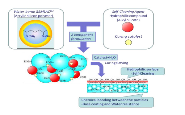
    [22] Sonoda T, Nakanishi Y, Hamamura T, et al. (2013) Development of self-cleaning top-coat for cool roof. Summaries of Technical Papers of 34th AIVC Conference: 268-270.
    [23] Fukaumi H, Hamamura T, Sonoda T (2015) Coating composition and coating film obtained from coating composition. European Patent Application, EP2821450A1.
    [24] Aoyama T, Sonoda T, Nakanishi Y, et al. (2017) Study on aging of solar reflectance of the self-cleaning high reflectance coating. Energ Buildings 157: 92-100. doi: 10.1016/j.enbuild.2017.02.021
    [25] Akbari H (2014) Advance in developing standards for accelerated aging of cool roofing materials. Summaries of Technical Papers of Roof Coating Manufacturers Association International Roof Coatings Conference.
    [26] Kakuta M (2004) Technology trends of anti-soiling and anti-bacterium. Tokyo: CMC Publishing.
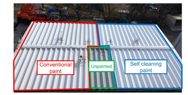
    [27] Aoyama T, Sonoda T, Takebayashi H (2017) Study on the influence of dirt and coating deterioration on aging of solar reflectance on high reflectance paint. AIJ Summaries of technical papers of annual meeting, Hiroshima, Japan, 395-396
    [28] Tamura M, Motohashi K, Shimizu R, et al. (2012) Study on performance of high reflectance paint for building Part7, Solar reflection after weathering test. Japan Society For Finishing Technology, Summaries of technical papers of annual meeting, Tokyo, Japan, 16-19.
    [29] Takebayashi H, Moriyama M (2012) Study on the estimation of solar reflectance reduction on cool coated corrugated roof. AIJ J Technol Des 18: 623-626.
    [30] JSTM J 6151 (2014) Method of measuring the solar reflectance of a flat roof in the field.
    [31] Murata Y, Sakai K, Miki K, et al. (2012) A study on the effect due to the reduction of absorbed solar radiation by cool painting, Part 1: improvement in estimated accuracy of field solar reflectivity measurement. Journal of JSES 38: 59-66.
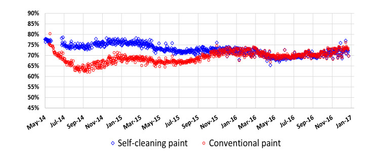
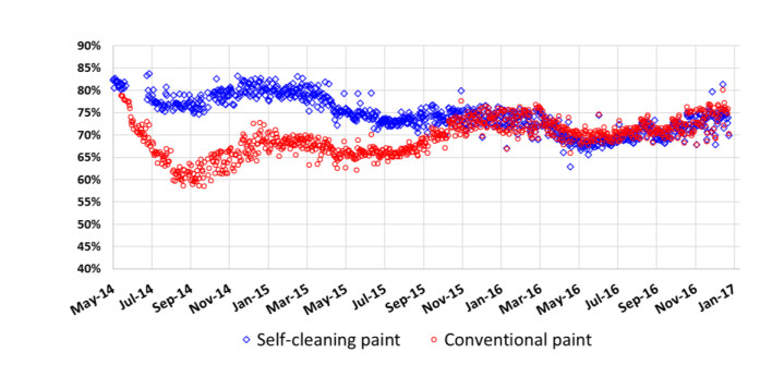
    [32] Takebayashi H, Tanabe J, Aoyama T, et al. (2017) Using field measurements to assess aging of self-cleaning high-reflectance paint. Int J Thermophys 38: 119.
    [33] Tsuruta T (1990) Applied Optics Ⅰ. Tokyo: Baifukan, 139-144.
  • This article has been cited by:

    1. Luis C. García-Naranjo, Rafael Ortega, Antonio J. Ureña, Invariant Measures as Obstructions to Attractors in Dynamical Systems and Their Role in Nonholonomic Mechanics, 2024, 29, 1560-3547, 751, 10.1134/S156035472456003X
  • Reader Comments
  • © 2019 the Author(s), licensee AIMS Press. This is an open access article distributed under the terms of the Creative Commons Attribution License (http://creativecommons.org/licenses/by/4.0)
通讯作者: 陈斌, bchen63@163.com
  • 1. 

    沈阳化工大学材料科学与工程学院 沈阳 110142

  1. 本站搜索
  2. 百度学术搜索
  3. 万方数据库搜索
  4. CNKI搜索

Metrics

Article views(4351) PDF downloads(459) Cited by(1)

Figures and Tables

Figures(7)  /  Tables(1)

/

DownLoad:  Full-Size Img  PowerPoint
Return
Return

Catalog