Review Special Issues

Probing the evolutionary history of epigenetic mechanisms: what can we learn from marine diatoms

  • Recent progress made on epigenetic studies revealed the conservation of epigenetic features in deep diverse branching species including Stramenopiles, plants and animals. This suggests their fundamental role in shaping species genomes across different evolutionary time scales. Diatoms are a highly successful and diverse group of phytoplankton with a fossil record of about 190 million years ago. They are distantly related from other super-groups of Eukaryotes and have retained some of the epigenetic features found in mammals and plants suggesting their ancient origin. Phaeodactylum tricornutum and Thalassiosira pseudonana, pennate and centric diatoms, respectively, emerged as model species to address questions on the evolution of epigenetic phenomena such as what has been lost, retained or has evolved in contemporary species. In the present work, we will discuss how the study of non-model or emerging model organisms, such as diatoms, helps understand the evolutionary history of epigenetic mechanisms with a particular focus on DNA methylation and histone modifications.

    Citation: Achal Rastogi, Xin Lin, Bérangère Lombard, Damarys Loew, Leïla Tirichine. Probing the evolutionary history of epigenetic mechanisms: what can we learn from marine diatoms[J]. AIMS Genetics, 2015, 2(3): 173-191. doi: 10.3934/genet.2015.3.173

    Related Papers:

    [1] Bing Liu, Gang Hu, Baolin Kang, Xin Huang . Analysis of a hybrid pest management model incorporating pest resistance and different control strategies. Mathematical Biosciences and Engineering, 2020, 17(5): 4364-4383. doi: 10.3934/mbe.2020241
    [2] Liping Wu, Zhongyi Xiang . A study of integrated pest management models with instantaneous and non-instantaneous impulse effects. Mathematical Biosciences and Engineering, 2024, 21(2): 3063-3094. doi: 10.3934/mbe.2024136
    [3] Zhenzhen Shi, Huidong Cheng, Yu Liu, Yanhui Wang . Optimization of an integrated feedback control for a pest management predator-prey model. Mathematical Biosciences and Engineering, 2019, 16(6): 7963-7981. doi: 10.3934/mbe.2019401
    [4] Wenjie Qin, Yue Xia, Yi Yang . An eco-epidemic model for assessing the application of integrated pest management strategies. Mathematical Biosciences and Engineering, 2023, 20(9): 16506-16527. doi: 10.3934/mbe.2023736
    [5] Dan Zhu, Qinfang Qian . Optimal switching time control of the hyperbaric oxygen therapy for a chronic wound. Mathematical Biosciences and Engineering, 2019, 16(6): 8290-8308. doi: 10.3934/mbe.2019419
    [6] Alhadi E. Alamir, Gomah E. Nenaah, Mohamed A. Hafiz . Mathematical probit and logistic mortality models of the Khapra beetle fumigated with plant essential oils. Mathematical Biosciences and Engineering, 2015, 12(4): 687-697. doi: 10.3934/mbe.2015.12.687
    [7] Urszula Ledzewicz, Shuo Wang, Heinz Schättler, Nicolas André, Marie Amélie Heng, Eddy Pasquier . On drug resistance and metronomic chemotherapy: A mathematical modeling and optimal control approach. Mathematical Biosciences and Engineering, 2017, 14(1): 217-235. doi: 10.3934/mbe.2017014
    [8] Xinli Hu, Wenjie Qin, Marco Tosato . Complexity dynamics and simulations in a discrete switching ecosystem induced by an intermittent threshold control strategy. Mathematical Biosciences and Engineering, 2020, 17(3): 2164-2178. doi: 10.3934/mbe.2020115
    [9] Wenjie Qin, Jiamin Zhang, Zhengjun Dong . Media impact research: a discrete SIR epidemic model with threshold switching and nonlinear infection forces. Mathematical Biosciences and Engineering, 2023, 20(10): 17783-17802. doi: 10.3934/mbe.2023790
    [10] Jiangtao Dai, Ge Guo . A leader-following consensus of multi-agent systems with actuator saturation and semi-Markov switching topologies. Mathematical Biosciences and Engineering, 2024, 21(4): 4908-4926. doi: 10.3934/mbe.2024217
  • Recent progress made on epigenetic studies revealed the conservation of epigenetic features in deep diverse branching species including Stramenopiles, plants and animals. This suggests their fundamental role in shaping species genomes across different evolutionary time scales. Diatoms are a highly successful and diverse group of phytoplankton with a fossil record of about 190 million years ago. They are distantly related from other super-groups of Eukaryotes and have retained some of the epigenetic features found in mammals and plants suggesting their ancient origin. Phaeodactylum tricornutum and Thalassiosira pseudonana, pennate and centric diatoms, respectively, emerged as model species to address questions on the evolution of epigenetic phenomena such as what has been lost, retained or has evolved in contemporary species. In the present work, we will discuss how the study of non-model or emerging model organisms, such as diatoms, helps understand the evolutionary history of epigenetic mechanisms with a particular focus on DNA methylation and histone modifications.


    In the integrated pest management, chemical control is one of the main control tactics, and the pesticides and other chemicals for the pest management are employed in reality [1,2,3,4]. The emergence of chemical synthetic insecticides has made great contributions to the control of some vector insects, agricultural pests and infectious diseases spread by them. At the same time, chemical pesticides are easy to operate and can control pests quickly and effectively. Therefore, in a long time at present and in the future, it is still a favorable weapon to fight vector insects and agricultural pests in rural areas. However, due to the high frequency and large-scale use of pesticides all over the world, long term accumulation leads to the occurrence and development of resistance and serious environmental pollution, which results in the decrease of the sensitivity of pests to pesticides, so they are not inhibited or poisoned by pesticides[5,6,7,8].

    Therefore, how to reduce or delay the resistance of pests to pesticides, how to make the pesticides play their role to the maximum extent, and how to reduce the impact of pesticides on the ecological environment are issues of agricultural administrative departments. The purpose of resistance management is to find appropriate ways to slow down and prevent the occurrence and development of pest resistance to pesticide, or restore resistant pest to a sensitive state. The key of resistance management is to reduce the selection pressure of pesticides on pests[9,10,11]. The development of pest resistance to pesticide is divided two types: external induced resistance and genetic resistance. The external induced resistance is that the pest developed the resistance to pesticide due to the large dosage and high frequency of pesticide spraying. Genetic resistance refers to the resistance generated by genetic inheritance of the resistance of the previous generation of pests to pesticides [12]. Since most of the pests that are sensitive to pesticides are killed during the use of pesticides, the surviving pests with pesticide resistance will pass on the resistance genes to the next generation. Therefore, with the change of generations, the proportion of pests carrying resistance genes becomes higher and higher, and the effect of pesticides gradually decreases, which seriously affects the success or failure of pest and disease control. In order to restrain the resistance of pest to pesticide, some principles have been proposed including rotation or switching between different types of pesticides, using biological control techniques, delaying the emergence of resistance, restoring the sensitivity of pests to pesticides and so on [13,14,15,16,17].

    Recently, pest management models with pest resistance to pesticide have been widely studied. Dobson and May combining population dynamics and genetics modelled the development of pest resistance to pesticide [18]. Liang et al. developed a continuous pest population growth model with both evolution of pesticide resistance and instantaneous pesticide applications, and studied the optimal time for switching between different kinds of pesticides under three different threshold levels [10]. Considering the growth of most pest population is not continuous, the novel discrete pest population models with the evolution of pest resistance to pesticide have been proposed and analyzed by Liang et al, who studied the effects of complex dynamical behaviour of pest population on pesticide switching strategies[11]. The genetic resistance was ignored and they only considered the external induced resistance in all of those studies.

    An interesting question is how to describe impulsive control strategies implemented within each generation when pests have non-overlapping generations, including impulsive release of natural enemies and spraying of pesticides. In order to solve this problem, some interesting modeling methods have been proposed recently. Tang et al. simplified hypothesis control strategy which is implemented at the beginning or the end of each generation [19]. Wang et al. first proposed a single population model with multiple impulsive pesticides applications within each generation, and then studied the existence and stability of the unique positive equilibrium[20]. Liang et al. proposed an analysis method of extended discrete model based on continuous logistic model under impulse perturbation to model the effects of single pesticide applications within each generation on populations growth[21].

    Once the pest resistance to pesticide is genetic, the questions are how to model the external induced resistance and genetic resistance in pest control model, and how to management the pest resistance to pesticide to achieve the purpose of pest control to solve those problems, according to the genetic laws and pesticide spraying, we modeled a pest resistance to pesticide model combine the external induced resistance and genetic resistance. Then we introduce the pest resistance to pesticide model into pest control models, the threshold conditions of pest eradication were discussed. For resistance management, we discussed the pesticide switching strategy, and the optimal switching time was investigated under the control strategy of one times pest control within each pest generation and multiple pest control within each pest generation. Moreover, the effects of the death rate of susceptible pests, the spraying times of pesticide within each generation, the dominance of resistance allele on the pesticide switching generations were studied.

    As described in the first part of the introduction, the development of pests' resistance on pesticide has a significant impact on pest control. To address those effects, we first investigate the evolution of pests' resistance, i.e.. we will analyze the development of pests' resistance from the perspective of gene inheritance and establish the development equation of pests' resistance. Moreover, the evolution of pests' resistance has been combined into the pest growth model.

    We assume that the pesticide resistance is determined by a single gene with two alleles $ R $ and $ S $. $ R $ denotes the resistance allele which represents the ability to survive on pesticide spraying. $ S $ denotes the susceptibility allele which represents the ability to survive with no resistance to the pesticide. According to Mendelian genetic law, we divide the pest population into three different types: homozygote resistant individuals $ RR $, homozygote susceptibles $ SS $ and heterozygotes $ RS $. In the presence of an application of pesticide, we denote $ W_{RR} $, $ W_{RS} $, $ W_{SS} $ are the fitness of $ RR $ type pest, the fitness of $ RS $ type pest and the fitness of $ SS $ type pest, respectively. Note that the fitness of an individual is independent of its genotype frequency [22], and we assume that pest individual is mated randomly. According to the hardy-weinberg principle [23], if the frequence of resistance allele is $ p_n $ and the frequence of susceptible allele is $ q_n $ in generation $ n $ (with $ p_n+q_n = 1 $), then the genotype frequencies in pests after selection are given by the following equations

    $ RR_n = \frac{W_{RR}p_n^2}{\overline{W}_n}, RS_n = \frac{W_{RS}2p_nq_n}{\overline{W}_n}, SS_n = \frac{W_{SS}q_n^2}{\overline{W}_n}, $

    where $ \overline{W}_n $ is the mean fitnesses with

    $ \overline{W}_n = p_n^2W_{RR}+2p_nq_nW_{RS}+q_n^2W_{SS}. $

    The averages fitnesses of the resistance allele $ R $ at generation $ n $ is

    $ {w}_n = p_nW_{RR}+q_nW_{RS}. $

    Consequently, the frequence of the resistance allele $ R $ in generation $ n+1 $ becomes

    $ p_{n+1} = \frac{p_n{w}_n}{\overline{W}_n} = \frac{p_n\left(p_nW_{RR}+q_nW_{RS}\right)}{\overline{W}_n}. $

    Submitting $ q_n = 1-p_n $, we have the evolution of pesticide resistance

    $ pn+1=p2n(WRRWRS)+pnWRSp2n(WSS2WRS+WRR)+pn(2WRS2WSS)+WSS.
    $
    (2.1)

    Note that this genetic model has been widely used in different fields [14,24,25,26,27,28].

    Table 1.  Parameters and presentation used in construction of the model.
    Parameters Presentation
    $ d_1 $ The mortality rate of susceptible pests
    $ h $ Dominance of pesticide resistance allele
    $ M $ Spray times within each generation
    $ p_0 $ Initial gene frequency
    $ r $ The intrinsic growth rate
    $ K $ The carrying capacity
    $ x_0 $ Initial population size of pests
    $ T $ The period of pesticide applications

     | Show Table
    DownLoad: CSV

    From Eq (2.1), it is obvious to see that $ p_n $ depends on the relative values of $ W_{RR} $, $ W_{RS} $ and $ W_{SS} $. Now we focus on deriving equations that represent the fitness of the three different genotypes: $ RR $, $ RS $, and $ SS $. We know that the death rate of pests strictly depends on the dosage of pesticide spraying. For simplification, we assume that the same dosage of pesticide is sprayed at each control event, and without loss of generality, we assume that one unit dose of pesticide is sprayed at each control event. Naturally, the homozygote susceptibles $ SS $ are assumed to die with a higher death rate $ d_1 $ $ (0\leq d_1\leq1) $ when a single pest control is carried out with one unit dose of pesticide is sprayed (Note that the different pesticides have different $ d_1 $, for convenience, we use $ d_1 $ as death rate in the whole study. For the specific pesticide, we only need to give specific value of $ d_1 $ in the following results). However, death rate is reduced by the level of dominance of pesticide resistance allele $ h $ $ (0\leq h\leq 1) $ in $ RS $ individuals, thus, the death rate of heterozygous individuals is $ (1-h)d_1 $ after one unit of sprayed pesticide. And the death rate of resistant individuals $ RR $ is $ d_2 $, for simplicity, we assume that the death rate of resistant individuals $ RR $ extremely low, that is $ d_2\approx 0 $. Consequently, the fitness of each genotype after pesticide is applied once within each generation is

    $ W_{RR} = W_{RR}^{(1)} = 1, $
    $ W_{RS} = W_{RS}^{(1)} = 1-(1-h)d_1, $
    $ W_{SS} = W_{SS}^{(1)} = 1-d_1. $

    In reality, farmers usually spray pesticides multiple times within each pest generation. In order to investigate the evolution of pests' resistance in this case, we assume that the pesticide is sprayed $ M $ times ($ M \geq 1 $) within each generation, and the fitness of each genotype after $ m- $times pesticide spraying in each generation is $ W_{RR}^{(m)} $, $ W_{RS}^{(m)} $, $ W_{SS}^{(m)} $, ($ m = 1, 2, ...M $). We know that the fitness of homozygote sensitives $ W_{SS} $ is $ W_{SS}^{(1)} = 1-d_1 $ for once pesticide spraying, $ W_{SS}^{(2)} = (1-d_1)^2 $ for $ 2- $times pesticide spraying, $ \cdots $, and the fitness of heterozygotes $ W_{RS} $ is $ W_{RS}^{(1)} = 1-(1-h)d_1 $ for once pesticide spraying, $ W_{RS}^{(2)} = (1-(1-h)d_1)^2 $ for $ 2- $times pesticide spraying$ \cdots $. Thus, the fitness of each genotype after spraying pesticide $ m $ times within each generation can be expressed as

    $ W_{RR}^{(m)} = 1, $
    $ W_{RS}^{(m)} = (1-(1-h)d_1)^m, $
    $ W_{SS}^{(m)} = (1-d_1)^m. $

    Thus, the frequence of genotypes after $ m $ times pesticide spraying in the $ n $th generation are given by the following equations

    $ SS_{n, m} = \frac{W_{SS}^{(m)}q_n^2}{\overline{W}_{n, m}}, \ \ RS_{n, m} = \frac{W_{RS}^{(m)}2p_nq_n}{\overline{W}_{n, m}}, \ \ RR_{n, m} = \frac{W_{RR}^{(m)}p_n^2}{\overline{W}_{n, m}}, $

    where $ \overline W_{n, m} $ is the mean fitness of the pest population after $ m $ times pesticide spraying in the $ n $th generation, which is given by

    $ \overline W_{n, m} = p_n^2W_{RR}^{(m)}+2p_nq_nW_{RS}^{(m)}+q_n^2W_{SS}^{(m)}. $

    And the averages fitnesses of the resistance allele $ R $ after $ m $ times pesticide spraying in the $ n $th generation is

    $ {w}_{n, m} = p_nW_{RR}^{(m)}+q_nW_{RS}^{(m)}. $

    Thus, the frequency of the resistance allele $ R $ in pests from $ n $th generation, to $ n+1 $th generation is

    $ pn+1=pnwn,M¯Wn,M=p2n(W(M)RRW(M)RS)+pnW(M)RSp2n(W(M)SS2W(M)RS+W(M)RR)+pn(2W(M)RS2W(M)SS)+W(M)SS.
    $
    (2.2)

    If the pesticide have completely kill rate to the homozygote sensitives (i.e., $ d_1 = 1 $ and $ W_{SS}^{(M)} = 0 $), then

    $ pn+1=pn(1W(M)RS)+W(M)RSpn(12W(M)RS)+2W(M)RS.
    $
    (2.3)

    Solving equation Eq (2.3) with initial gene frequency $ p_0 $, we have

    $ pn=β(p01)(W(M)RS)np0+β(p01)(W(M)RS)np0+β,
    $
    (2.4)

    where $ \beta = \frac{W_{RS}^{(M)}}{2W_{RS}^{(M)}-W_{RR}^{(M)}} $.

    In the next section, calculating the $ n $ is important to investigate the optimal generation for switching pesticide. From Eq (2.4), we can get

    $ n=logW(M)RS(p0β)(pn1)(p01)(pnβ).
    $
    (2.5)

    Now we consider the general case (i.e., $ W_{SS}^{(M)}\neq0 $). In order to obtain $ p_n $ or $ n $, we calculate the amount of change in gene frequency per generation by using Haldance' method [29], i.e..

    $ pn=pn+1pn=pn(1pn)(pn(1W(M)RS)+(1pn)(W(M)RSW(M)SS))¯Wn,M.
    $
    (2.6)

    We further assume that gene frequency is very low [30], its rate of change per generation could be given by

    $ dpndn=pn(1pn)(pn(1W(M)RS)+(1pn)(W(M)RSW(M)SS))¯Wn,M.
    $
    (2.7)

    In order to calculate $ n $, we divide it into three cases:

    Case 1: $ R $ is completely dominant gene in $ RS $, i.e., $ h = 1 $ [31].

    Integrating Eq (2.7) with the initial condition $ p_0 $, we have

    $ n=[11W(M)SS(ln(p01pn1(pnp0)W(M)SS)+pnp0(p01)(pn1))].
    $
    (2.8)

    Case 2: $ R $ is completely recessive gene in $ RS $, i.e., $ h = 0 $ [31].

    Integrating Eq (2.7) with the initial condition $ p_0 $, we can get

    $ n=[11W(M)SS(ln(p01pn1(pnp0)W(M)SS)+W(M)SS(pnp0)p0pn)].
    $
    (2.9)

    Case 3: $ R $ is incomplete dominant or incomplete recessive gene in $ RS $, i.e., $ 0 < h < 1 $.

    Integrating Eq (2.7) with the initial condition $ p_0 $, we can get

    $ n=[ln((pnp0)D(pn1p01)E(GnG0)F)],
    $
    (2.10)

    where $ {D} = \frac{W_{SS}^{(M)}}{W_{RS}^{(M)}-W_{SS}^{(M)}} $, $ {E} = -\frac{1}{1-W_{RS}^{(M)}} $, $ {F} = \frac{{W_{RS}^{(M)}}^2-W_{SS}^{(M)}}{(1-W_{RS}^{(M)})(W_{RS}^{(M)}-W_{SS}^{(M)})} $ and $ {G}_n = (1-2W_{RS}^{(M)}+W_{SS}^{(M)})p_n+W_{RS}^{(M)}-W_{SS}^{(M)} $. $ [a] $ denotes the greatest integer no larger than $ a $.

    Next, we investigate the effects of death rate of pesticide for homozygote susceptibles ($ d_1 $) and the spraying times ($ M $) on the frequence of resistance ($ p_n $). Because of the highly nonlinearity of Eq (2.10), we only focus on the effects in case 1 and case 2 theoretically, and for case 3, we just carry out some numerical simulations.

    For case 1, i.e.. $ R $ is completely dominant gene in $ RS $, differentiating Eq (2.8) with respect to $ d_1 $ and $ M $ respectively, we have

    $ \frac{\partial p_n}{\partial d_1} = \frac{MnW_{SS}^{(M-1)}+MW_{SS}^{(M-1)}\ln\frac{p_n}{p_0}}{\frac{1}{1-p_n}+W_{SS}^{(M)}\frac{1}{p_n}+\frac{1}{(p_n-1)^2}} \gt 0, $
    $ \frac{\partial p_n}{\partial M} = \frac{-W_{SS}^{(M)}n\ln W_{SS}^{(1)}-W_{SS}^{(M)}\ln W_{SS}^{(1)}\ln\frac{p_n}{p_0}}{\frac{1}{1-p_n}+W_{SS}^{(M)}\frac{1}{p_n}+\frac{1}{(p_n-1)^2}} \gt 0. $

    For case 2, i.e.. $ R $ is completely recessive gene in $ RS $, differentiating Eq $ (2.9) $ with respect to $ d_1 $ and $ M $ respectively, we have

    $ \frac{\partial p_n}{\partial d_1} = \frac{MnW_{SS}^{(M-1)}+MW_{SS}^{(M-1)}\ln\frac{p_n}{p_0}+MW_{SS}^{(M-1)}(\frac{1}{p_0}-\frac{1}{p_n})}{\frac{1}{1-p_n}+W_{SS}^{(M)}\frac{1} {p_n}+\frac{W_{SS}^{(M)}}{p_n^2}} \gt 0, $
    $ \frac{\partial p_n}{\partial M} = \frac{-W_{SS}^{(M)}n\ln W_{SS}^{(1)}-W_{SS}^{(M)}\ln W_{SS}^{(1)}\ln\frac{p_n}{p_0}-W_{SS}^{(M)}\ln W_{SS}^{(1)}\ln(\frac{1}{p_0}-\frac{1}{p_n})}{\frac{1}{1-p_n}+W_{SS}^{(M)}\frac{1}{p_n}+\frac{W_{SS}^{(M)}}{p_n^2}} \gt 0. $

    From the above formulas, we can see that $ p_n $ is an increasing function with respect to $ d_1 $ and $ M $ in both case 1 and case 2. That is, decreasing the death rate of susceptible pests or decreasing the spraying times of pesticide in each generation can decrease the values $ p_n $. In order to show in more detail how the level of dominance of pesticide resistance allele $ h $, the mortality rate $ d_1 $ and $ M $ affect evolution of pesticide resistance, we analyze those by numerically simulation in Figure 1. From Figure 1 (a) and (c), we can see that the higher the efficiency of the pesticides (i.e. the higher mortality rate), the faster the resistance development is. From Figure 1 (b) and (d), we can see that the more times of the pesticide spraying in one generation, the faster the resistance development is.

    Figure 1.  The effect of the mortality rate of susceptible pests $ d_1 $ and spray times $ M $ on $ p_n $. (a)–(b) $ R $ is completely recessive gene in $ RS $, (c)–(d) $ R $ is completely dominant gene in $ RS $, (e)–(f) $ R $ is incomplete dominant or incomplete recessive gene in $ RS $ and $ p_0 = 0.0001 $.

    If we fix the frequence of resistance, then we want to know how the death rate ($ d_1 $), spraying times ($ M $) and the level of dominance of pesticide resistance ($ h $) on generation ($ n $) which reach to fixed resistance level. For this purpose, we carry out the sensitivity analysis of $ n $ in Figure 2. In Figure 2, we fix $ p_n = 50\% $, and we can see that the higher the efficiency of the pesticides is (i.e., the higher mortality rate), the faster of the pest population reaches the fixed resistance level; The more times of the pesticide sprayed in one generation, the faster of the pest population reaches the fixed resistance level; The higher the level of dominance of pesticide resistance, the faster of the pest population reaches the fixed resistance level.

    Figure 2.  The effect of the mortality rate $ d_1 $ and spraying times $ M $ on $ n $, with the variation of $ h $ from $ 0 $ to $ 1 $ and $ p_0 = 0.005 $.

    Throughout this study, the pest population is assumed to grow logistically within each generation $ [n, n+1] $,

    $ dx(t)dt=rx(t)(1x(t)K),ntn+1,n=0,1,2,...,
    $
    (2.11)

    where $ x(t) $ is the density of the pest population at time $ t $, $ r $ denotes the intrinsic growth rate and $ K $ represents the carrying capacity.

    In reality, people usually spray pesticide within a fairly short period, so it's reasonable to assume that the density of pests can be reduced instantaneously once the chemical control tactics are applied. Therefore, the impulsive hybrid model based on Eq $ (2.11) $ can be employed to depict this control measure.

    If the pesticides is applied at time $ n+\tau_m $ ($ 0\leq \tau_m \leq1 $) with an instantaneous killing rate $ D_{n, m} $, then we have

    $ {dx(t)dt=rx(t)(1x(t)K),tn+τm,x(n+τm)+=(1Dn,m)x(n+τm),t=n+τm,Dn,m=d1SSn,m+(1h)d1RSn,m.
    $
    (2.12)

    From the former section, we have

    $ Dn,m=d1SSn,m+(1h)d1RSn,m=d1W(m)SSq2n+2(1h)d1W(m)RSpnqn¯Wn,m=p2na(m)+pnb(m)+c(m)p2na(m)1+pnb(m)1+c(m)1,
    $
    (2.13)

    with

    $ c^{(m)} = d_1W_{SS}^{(m)}, b^{(m)} = 2(1-h)d_1W_{RS}^{(m)}-2c^{(m)}, a^{(m)} = c^{(m)}-2(1-h)d_1W_{RS}^{(m)}, $

    and

    $ c_1^{(m)} = W_{SS}^{(m)}, b_1^{(m)} = 2W_{RS}^{(m)}-2c_1^{(m)}, a_1^{(m)} = c_1^{(m)}-2W_{RS}^{(m)}+1. $

    It is clear that the instantaneous killing rate $ D_{n, m} $ decreases as pesticide resistance develops.

    In this section, we assume that once control is implemented within each pest generation. We then investigate how to switch pesticides and manage the development of genetic resistance such that the pest population can be eventually eliminated or maintained at a density below EIL. In order to investigate those questions, we propose two different switching strategies, and investigate the optimal switching times under once control within each generation.

    We assume that pesticide was used once within each generation at time $ n+\tau_1 $ ($ 0\leq\tau_1\leq1 $) in $ n $th generation. The model Eq $ (2.12) $ becomes

    $ {dx(t)dt=rx(t)(1x(t)K),tn+τ1,x(n+τ1)+=(1Dn))x(n+τ1),t=n+τ1,Dn=d1SSn,1+d1(1h)RSn,1,
    $
    (3.1)

    where $ D_{n} = D_{n, 1} $. Solving Eq $ (3.1) $ within $ [n, n+1] $, we have

    $ x(t) = \frac{K x_ne^{r(t-n)}}{k+ x_n(e^{r(t-n)}-1)}, \ \ n\leq t\leq n+\tau_1, $
    $ x(t) = \frac{K x(n+\tau_1)^+e^{r(t-n-\tau_1)}}{K+ x(n+\tau_1)^+(e^{r(t-n-\tau_1)}-1)}, \ \ n+\tau_1\leq t\leq n+1. $

    Thus, we have

    $ x(n+\tau_1)^+ = \frac{K x_ne^{r\tau_1}(1-D_{n})}{K+ x_n(e^{r\tau_1}-1)} $

    and

    $ x(n+1)=Ker(1Dn)x(n)K+(erτ1Dn+er(1Dn)1)x(n).
    $
    (3.2)

    Denote $ x(n) = x_n $, then we have the following iteration equation from $ n $th generation to $ n+1 $th generation

    $ xn+1=Ker(1Dn)xnK+(erτ1Dn+er(1Dn)1)xn,
    $
    (3.3)

    which is a non-autonomous Beverton-Holt difference equation, i.e. the so-called extended Beverton-Holt model. For more details of extended Beverton-Holt model, please see the references [32,33,34,35,36,37].

    According to the properties of the extended Beverton-Holt model, we have that if $ e^r(1-D_{n}) < 1 $, then the zero solution of Eq $ (3.3) $ is globally asymptotically stable. Consequently, we can define the threshold value $ R_n $ as

    $ Rn=er(1Dn),
    $
    (3.4)

    where $ D_{n} $ can be calculated by Eq $ (2.13) $. Thus, the pest population will be eradicated if $ R_n < 1 $ for all $ n = 0, 1, 2, \cdots $.

    Note that $ R_n $ is dynamic and depends on $ D_{n} $. We can see that $ D_{n} $ is a monotonic decreasing function of $ n $. Therefore, as the pest generations increases, the threshold value $ R_n $ increases and exceeds one, resulting in pest resurgence and outbreaks.

    In Figure 3, we simulate the threshold $ R_n $ with different level of dominance of pesticide resistance allele in $ RS $ ($ h $) and the mortality rate ($ d_1 $), which reveal that $ R_n $ is an increasing function with respect to $ n $, and will exceed 1 after several pesticide pesticide applications. From Figure 3 (a), we can see that the greater of $ h $ is, the faster growth of $ R_n $ is. This is because that the higher of the level of dominance of pesticide resistance allele in $ RS $ is, the faster development of the pests' resistance is. All those confirm that the pest population will be resurgence and outbreaks as the pesticide resistance evolution. From Figure 3 (b), it is obvious that the effects of mortality rates $ d_1 $ on $ R_n $ are more complicated with the development of time $ n $. The bigger $ d_1 $ is, the smaller $ R_n $ is, when $ n $ is small. And with the increase of n, the effects of mortality rates $ d_1 $ on $ R_n $ is changed, the bigger $ d_1 $ is, the smaller $ R_n $ is. This is due to that in the early stages of the pest control, the more dosage of pesticide is sprayed, the higher of the mortality rate is, and the pest population is more easy to control with the high efficiency of pesticide. With the increasing of $ n $, the pest control times is increasing, and the pest's resistance is developed, which the results is the decline in efficiency of pesticide, and the pests' outbreak.

    Figure 3.  The effects of the level of dominance of pesticide resistance allele $ h $ and the mortality rate $ d_1 $ on the $ R_n $. The other parameters are given as follows: $ r = 0.65 $, $ p_0 = 0.0001 $; (a): $ d_1 = 0.7 $; (b): $ h = 0.65 $.

    In order to prevent pest population outbreaks and restrain the development of pesticide resistance, farmers usually switch some different type pesticide. And what is the optimal switching time with the aim of eradication of pest population. For this aim, we only need the threshold $ R_n $ below one for all $ n = 0, 1, 2, \cdots $. Therefore, farmers need to switch the pesticide before the threshold value $ R_n $ goes to one. Without loss of generality, we assume that the threshold value $ R_n $ will increase and exceed the unit after $ n_1 $th generation i.e

    $ n_1 = max\{n:R_n\leq1\}, $

    and the optimal switching time is $ n_1 $, or the maximum number of one type of pesticide spraying is $ n_1+1 $ (note that the first pesticide application is at time $ n = 0 $). That is, after $ n_1+1 $ times pesticide spraying, farmers should switching another type of pesticide.

    In order to determine $ n_1 $ analytically, we let $ R_n = 1 $, then

    $ 1-D_{n} = e^{-r}, $
    $ n_1 = [\{n:1-D_{n} = e^{-r}\}]. $

    From Eq $ (2.13) $, we can get

    $ 1Dn=p2n(a(1)1a(1))+pn(b(1)1b(1))+c(1)1c(1)p2na(1)1+pnb(1)1+c(1)1=er.
    $
    (3.5)

    That is

    $ p2n(a(1)1(1er)a(1))+pn(b(1)1(1er)b(1))+c(1)1(1er)c(1)=0.
    $
    (3.6)

    In order to solve Eq (3.6), we define the function $ f(x) $ as follows

    $ f(x)=Ah,d1x2+Bh,d1x+Cd1,(0x1),
    $
    (3.7)

    where

    $ {A}_{h, d_1} = a_1^{(1)}(1-e^{-r})-a^{(1)} = d_1(-2h^2d_1+h(2e^{-r}-4+4d_1)+2-d_1-e^{-r}), $
    $ {B}_{h, d_1} = b_1^{(1)}(1-e^{-r})-b^{(1)} = 2hd_1(hd_1+(2-2d_1-e^{-r})), $

    and

    $ {C}_{d_1} = c_1^{(1)}(1-e^{-r})-c^{(1)} = (1-d_1)(1-d_1-e^{-r}). $

    The Eq (3.6) becomes to $ f(p_n) = 0 $. Now we solve this equation with respect to $ p_{n} $, and substituting $ p_{n} = p_{n_1} $ into Eq $ (2.5) $ or Eqs $ (3.10) $–$ (2.10) $, we can obtain the optimal switching time $ n_1 $ under different cases.

    The $ p_{n_1} $ can be defined as follows:

    $ p_{n_1} = \left\{Bh,d1+B2h,d14Ah,d1Cd12Ah,d1,ifCd1<0andAh,d10,Cd1Bh,d1,ifCd1<0andAh,d1=0,Bh,d1Ah,d1,ifCd1=0,Bh,d1<0andAh,d1>0.
    \right. $

    The detailed calculation of the $ p_{n_1} $ is provided in Appendix A.

    Now we turn our attention to the effect of the timing of pesticide applications $ \tau_1 $ on the density of pest population $ x_n $. From Eq $ (3.3) $ we have the following iteration equation

    $ xn=KNnx0K+Snx0,
    $
    (3.8)

    where

    $ N_{n} = e^{nr}\prod\limits_{j = 0}^{n-1}(1-D_j) $

    and

    $ S_n = \left\{erτ1D0+Nn1,                     n=1,erτ1D0+n1i=1(er(i+τ1)Dii1j=0(1Dj))+Nn1,  n>1.
    \right. $

    It's easy to see that $ x_n $ is a decreasing function with respect to $ \tau_1 $, this means that the later of pest control is, the smaller of pest population density is, and more benefit to pest control. In Figure 4, we simulate the development of $ x_n $ with respect to $ n $ under different $ \tau_1 $. From Figure 4, we can see that the later insecticide spraying time is, the smaller the population density is, and we also see that the density of pest population $ x_n $ is decreasing at the beginning of pest control, and then the density of pest population $ x_n $ is increasing after some pesticide applications. The reason is that with the increasing of number of pesticide sprayings, the pesticide resistance is developed, and consequently, the density of pest population can not decrease any more, instead, it increases rapidly, even exceeds the EIL.

    Figure 4.  The effects of the time factor $ \tau_1 $ on the density of $ x_n $ predicated by Eq $ (3.3) $ for $ \tau_1 = 0.1 $, $ \tau_1 = 0.5 $, $ \tau_1 = 0.9 $, respectively. The parameter values are fixed as follows: $ r = 0.65 $, $ \eta = 80 $, $ x_0 = 20 $, $ d_1 = 0.55 $, $ h = 0.65 $, $ p(1) = 0.0001 $, $ EIL = 35 $.

    As mentioned in the introduction, the pre-set goal of the pest management is to control the density of the pest below the EIL. However, the pest population will exceed the EIL eventually if only one type of pesticide is used (i.e. do not switch pesticides), see Figure 4. Thus, in order to successfully control the density of pest population below the EIL, farmers should switch another kind of pesticide before the density of pest population reach to EIL. In this subsection, we will investigate the optimal switching time with EIL as switching guide.

    In there, we assume that the pest population density exceeds EIL for the first time in the $ n_2+1 $th generation.This indicates that $ x_{n_2}\leq EIL $ and $ x_{n_2+1} > EIL $, that is the optimal switching generation is $ n_2+1 $.

    From Eq $ (3.3) $, we have

    $ xn2+1=Ker(1Dn2)xn2K+(erτ1Dn2+er(1Dn2)1)xn2>EIL,
    $
    (3.9)

    and we can get

    $ (Ker(1Dn2)EIL(erτ1Dn2+er(1Dn2)1))xn2>KEIL.
    $
    (3.10)

    It follows from $ x_{n_2}\leq EIL $ that

    $ K e^r(1-D_{n_2})-EIL(e^{r\tau_1}D_{n_2}+e^r(1-D_{n_2})-1) \gt K, $

    then

    $ D_{n_2} \lt E_1, $

    where $ E_1 = \frac{(e^r-1)(K-EIL)}{e^r(K-EIL)+EIL e^{r\tau_1}} $. It is easy to see that $ E_1 $ is decreasing as $ \tau_1\rightarrow1 $. This implies that $ n_2 $ is increasing as $ \tau_1\rightarrow1 $, in other words, under the EIL guided switching strategy, the number of the same pesticide used increases with the increasing of $ \tau_1 $.

    Substituting Eq $ (3.8) $ into Eq $ (3.10) $, we have

    $ \left(K e^r(1-D_{n_2})-EIL(e^{r\tau_1}D_{n_2}+e^r(1-D_{n_2})-1)\right)\frac{K N_{n_2}x_0}{K+S_{n_2} x_0} \gt K EIL, $

    thus

    $ Zn2>EILK+x0EILD0erτ1EILx0x0,
    $
    (3.11)

    where $ Z_{n_2} = (K-EIL)N_{n_2+1}-EIL\sum_{i = 1}^{n_2}\left(e^{r(i+\tau_1)}D_i\prod_{j = 0}^{i-1}(1-D_j)\right) $.

    Therefore,

    $ n2=[{l|Zl=EILK+x0EILD0erτ1EILx0x0}].
    $
    (3.12)

    In order to understand these two different switching strategies more intuitively, we draw some numerical simulations in the Figure 5. From Figure 5 (a) we can see that under the $ R_n $ guided switching strategy the pest population will be eradicated completely after several pesticide switches, where $ n_1 = 3 $. That is after four pesticide applications of one kind of pesticide (note that the first pesticide application is at time $ n = 0 $), the farmers must switch to another kind of pesticide to eradicate the pest quickly. From Figure 5 (b) we can see that under the EIL guided switching strategy pest control will tends to periodic control after a certain number of pesticide switches. This is due to the development of resistance of pest on the same type pesticide, the density of pest population will exceed EIL after some numbers of the same type pesticide spraying, under the EIL guided switching strategy pest control, farmers should switching another type of pesticide at the last number of pesticide spraying before the density of pest population reach to EIL (we assume that the pest population has the same development of pesticide resistance on different type of pesticide), due to the same process of pesticide resistant evolution and pest control period, the pest control will tends to periodic control under this switching strategy.

    Figure 5.  Illustrations of two different switching strategies.The parameter values are fixed as follows:$ r = 0.6 $, $ K = 50 $, $ x_0 = 20 $, $ \tau_1 = 0.9 $, $ d_1 = 0.65 $, $ h = 0.65 $, $ p_0 = 0.005 $, $ EIL = 35 $. (a) Numerical simulations of Eq $ (3.3) $ with several pesticides switches guided by threshold condition; (b) Numerical simulations of Eq $ (3.3) $ with several pesticides switches guided by the EIL.

    In reality, the pesticide is sprayed for multiple times in each generation to control pest. Therefore, in this section, we developed an extended discrete single population model with multiple impulsive chemical control within each generation, and then investigate the optimal generation for switching pesticides.

    We assume that the pesticides are applied $ M $ times within each generation, that is to see, there exist $ \tau_m (m = 1, 2\cdots, M) $ with $ n\leq n+\tau_1\leq n+\tau_2\leq\cdots\leq n+\tau_M\leq n+1 $, such that the pesticides have been applied at $ n+\tau_m $ with a proportion $ D_{n, m} $ of the pest being killed. We have

    $ {dx(t)dt=rx(t)(1x(t)K)tn+τm,x(n+τm)+=(1Dn,m)x(n+τm)t=n+τm,Dn,m=d1SSn,m+(1h)d1RSn,m.
    $
    (4.1)

    For convenience, we denote $ D_{n, 0} = 0 $. Therefore, by employing the same methods proposed before, we have the following extended discrete single population model with multiple impulsive chemical control within each generation

    $ xn+1=erKMm=1(1Dn,m)xnK+(Mm=1(erτmDn,mmi=1(1Dn,i1))+erMm=1(1Dn,m)1)xn.
    $
    (4.2)

    In particular, if $ M = 1 $ then we have $ \sum_{m = 1}^{M}(e^{r\tau_m}D_{n, m}\prod_{j = 1}^{m}(1-D_{n, j-1})) = e^{r\tau_1}D_{n} $.

    For simplicity, we assume that the pesticides are sprayed periodically within each generation, which satisfies $ \tau_{m+1}-\tau_{m} = T $ for m = 1, 2..., M and $ 0 < T\leq\frac{1-\tau_1}{M-1} $, thus we can get

    $ xn+1=KλnxnK+(μn+λn1)xn,
    $
    (4.3)

    with $ \lambda_n = e^r\prod_{m = 1}^{M}(1-D_{n, m}) $ and $ \mu_n = \sum_{m = 1}^{M}(e^{r(\tau_1+(m-1)T)}D_{n, m}\prod_{i = 1}^{m}(1-D_{n, i-1})) $. Note that this is the extended Beverton-Holt model, and if $ e^r\prod_{m = 1}^{M}(1-D_{n, m}) < 1 $, the population size is gradually reduced and becomes extinct eventually. We can define the dynamic threshold value $ R_n^M $ as follows:

    $ R_n^M = e^r\prod\limits_{m = 1}^{M}(1-D_{n, m}), $

    that is, if $ R_n^M < 1 $, the population size is gradually reduced and becomes extinct eventually.

    In order to analyse the effects of the spraying times $ M $ of pesticides in each generation on the threshold value $ R_n^M $, we simulate the threshold value $ R_n^M $ with different spraying times $ M $ in Figure 6. From Figure 6, we can see that $ R_n^M $ is a decreasing function with respect to $ M $, that is, the more spraying times in each generation is, the later of the density of pest population reaching to $ R_n^M $ is.

    Figure 6.  The effects of the spraying $ M $ of pesticide in each generation on the threshold value $ R_n^M $. The parameters value are fixed as follows: $ r = 0.4 $, $ d_1 = 0.6 $, $ h = 0.75 $, $ p_0 = 0.0001 $.

    From Figure 6, we can also see that the density of pest population will reach to the threshold after several times of spraying pesticide, due to the development of pesticide resistance. Therefore, in order to eradicate pest population, the alternative choice is to switch another pesticide after the using of one pesticide for several times. In the following, we will discuss the optimal switching time.

    Note that, in order to eradicate the pests population, the threshold value $ R_n^M $ should below one for all $ n = 0, 1, 2, \cdots $. Therefore, it's necessary to switch the pesticides before the threshold value $ R_n^M $ reach to one. Here, we assume that the threshold value reach or exceed to 1 firstly after pest control in $ n_3 $th generation, i.e..

    $ n_3 = max\{n:R_n^M\leq1\}, $

    and the optimal generation for switching pesticides is $ n_3 $. In order to determine $ n_3 $ analytically, we let $ R_n^M = 1 $, that is

    $ RMn=erMm=1(1Dn,m)=1,
    $
    (4.4)

    or

    $ n_3 = [\{n:\prod\limits_{m = 1}^{M}(1-D_{n, m}) = e^{-r}\}]. $

    From Eq $ (2.13) $, we have

    $ 1Dn,m=1p2na(m)+pnb(m)+c(m)p2na(m)1+pnb(m)1+c(m)1=p2na(m+1)1+pnb(m+1)1+c(m+1)1p2na(m)1+pnb(m)1+c(m)1,
    $

    submitting the former Eq (4.4), we get

    $ Mm=1(1Dn,m)=p2na(M+1)1+pnb(M+1)1+c(M+1)1p2na(1)1+pnb(1)1+c(1)1=er.
    $
    (4.5)

    Letting

    $ g(x)=AMh,d1x2+BMh,d1x+CMd1,
    $
    (4.6)

    with

    $ AMh,d1=a(M+1)1era(1)1=(1d1)M+12(1(1h)d1)M+1+1erd1(12h),
    $
    $ BMh,d1=b(M+1)1erb(1)1=2(1(1h)d1)M+12(1d1)M+1er2d1h=2hd1((M+1)(1d1)Mer)+M+1i=2(2(hd1)iCiM+1(1d1)M+1i),
    $

    where $ \mathbb{C}_{M+1}^i = \frac{(M+1)!}{i!(M+1-i)!} $ is combinatorial number, and

    $ CMd1=c(M+1)1erc(1)1=(1d1)((1d1)Mer).
    $

    Then Eq $ (4.5) $ becomes $ g(p_n) = 0 $. Solving $ g(p_n) = 0 $ with respect to $ p_n $ we can obtain $ p_{n_3} $, with

    $ p_{n_3} = \left\{BMh,d1+BMh,d124AMh,d1CMd12AMh,d1,ifCMd1<0andAMh,d10,CMd1BMh,d1,ifCMd1<0andAMh,d1=0,BMh,d1AMh,d1,ifCMd1=0,BMh,d1<0andAMh,d1>0
    \right. $

    The detailed calculation of the $ p_{n_3} $ is provided in Appendix B. We substitute $ p_{n_3} $ into Eq $ (2.5) $ or Eqs $ (3.10) $–$ (2.10) $, and we can obtain the optimal switching time $ n_3 $ under different cases.

    In the following, we address how the $ x_{n} $ varies as the parameters $ \tau_1 $ and $ T $ change, which are quite important for pesticide applications. Firstly, by induction, we can get the recursion formula for $ x_{n} $ of Eq $ (4.3) $ as follows:

    $ xn=KNMnx0K+SMnx0,
    $
    (4.7)

    where

    $ N_n^M = e^{rn}\prod\limits_{j = 0}^{n-1}\prod\limits_{m = 1}^M(1-D_{j, m}), $
    $ S_n^M = \left\{Mm=1(er(τ1+(m1)T)D0,mm1l=0(1D0,l))+NMn1,        n=1,Mm=1(er(τ1+(m1)T)D0,mm1l=0(1D0,l))+δn+NMn1,  n>1,
    \right. $

    with

    $ \delta_n = \sum\limits_{i = 1}^{n-1}\left(\sum\limits_{m = 1}^M\left(e^{r(i+\tau_1+(m-1)T)}D_{i, m}(\prod\limits_{j = 0}^{m-1}(1-D_{i, j}))(\prod\limits_{k = 0}^{i-1}\prod\limits_{m = 1}^{M}(1-D_{k, m}))\right)\right). $

    From Eq $ (4.7) $ we can see that $ x_n $ is a decreasing function with respect to $ \tau_1 $ and $ T $, which means that the longer of period or the later of pesticide spraying is, the more benefit to pest control.

    In this subsection, we focus on the control tactics of $ EIL $. That is farmers should control pest when the density of pest population reach to $ EIL $. As the former states, because of the resistance of pesticide, spraying one type of pesticide could not maintain the density of pest population below the $ EIL $. Thus after some times of one type of pesticide spraying, farmers should switch another type of pesticides.

    We assume that after the $ n_4 $th generation, farmers should switch another type of pesticide, which means that $ x_{n_4}\leq EIL $ and $ x_{n_4+1} > EIL $, that is, the optimal switching generation is $ n_4+1 $. In order to find the $ n_4 $, we let $ x_{n_4+1} > EIL $. From Eq $ (4.3) $, we have

    $ xn4+1=Kλn4xn4K+(μn4+λn41)xn4>EIL,
    $
    (4.8)

    then we can get

    $ (λn4K(μn4+λn41)EIL)xn4>EILK.
    $
    (4.9)

    Due to $ x_{n_4}\leq EIL $, from Eq (4.9), we can get

    $ λn4K(μn4+λn41)EIL>K.
    $
    (4.10)

    From Eq $ (2.13) $, we can get

    $ \lambda_{n_4} = e^r\prod\limits_{m = 1}^{M}(1-D_{n_4, m}) = \frac{e^{r}(p_{n_4}^2a_1^{(M+1)}+p_{n_4}b_1^{(M+1)}+c_1^{(M+1)})}{p_{n_4}^2a_1^{(1)}+p_{n_4}b_1^{(1)}+c_1^{(1)}}, $

    and $ \mu_{n_4} $ can be calculated as follows

    $ \mu_{n_4} = \sum\limits_{m = 1}^{M}(e^{r(\tau_1+(m-1)T)}D_{n_4, m}\prod\limits_{i = 1}^{m}(1-D_{n_4, i-1})) = \frac{p_{n_4}^2(\theta_1-2\theta_2)+p_{n_4}(2\theta_2-2\theta_1)+\theta_1}{p_{n_4}^2a_1^{(1)}+p_{n_4}b_1^{(1)}+c_1^{(1)}}, $

    with

    $ \theta_1 = d_1\sum\limits_{m = 1}^Me^{r(\tau_1+(m-1)T)}W_{SS}^{(m)} = \frac{e^{r\tau_1}W_{SS}^{(1)}d_1(1-e^{rTM}W_{SS}^{(M)})}{1-e^{rT}W_{SS}^{(1)}}, $
    $ \theta_2 = d_1(1-h)\sum\limits_{m = 1}^Me^{r(\tau_1+(m-1)T)}W_{RS}^{(m)} = \frac{e^{r\tau_1}W_{RS}^{(1)}(1-h)d_1(1-e^{rTM}W_{RS}^{(M)})}{1-e^{rT}W_{RS}^{(1)}}, $

    thus Eq $ (4.10) $ can be rewritten as follows

    $ p2n4H1+pn4H2+H3p2n4a(1)1+pn4b(1)1+c(1)1>KEIL,
    $
    (4.11)

    where

    $ H_1 = a_1^{(M+1)}e^r(K- EIL)-(\theta_1-2\theta_2) EIL, $
    $ H_2 = b_1^{(M+1)}e^r(K- EIL)-(2\theta_2-2\theta_1) EIL, $
    $ H_3 = c_1^{(M+1)}e^r(K- EIL)-\theta_1 EIL. $

    This indicates that $ p_{n_4} $ should be satisfied

    $ pn4(ˆAMh,d1pn4+ˆBMh,d1)>ˆCMd1,
    $
    (4.12)

    where $ \widehat{A}_{h, d_1}^M = H_1-(K- EIL)a_1^{(1)} $, $ \widehat{B}_{h, d_1}^M = H_2-(K- EIL)b_1^{(1)} $ and $ \widehat{C}_{d_1}^M = (K- EIL)c_1^{(1)}-H_3. $

    Substituting Eq $ (4.7) $ into Eq $ (4.9) $ gives

    $ Y_{n_4} \gt \frac{EILK+x_0EIL\sum_{m = 1}^M\left(e^{r(\tau_1+(m-1)T)}D_{0, m}\prod_{l = 0}^{m-1}(1-D_{0, l})\right)-x_0EIL}{x_0}, $

    with $ Y_{n_4} = (K-EIL)N_{n_4+1}^M-EIL\delta_{n_4+1} $. Thus, we have

    $ n4=[{l|Yl=EILK+x0EILMm=1(er(τ1+(m1)T)D0,mm1l=0(1D0,l))x0EILx0}].
    $
    (4.13)

    There are many factors to cause the resistance of pest to pesticide. The main factors are the external factor (i.e. the high frequency and large doses spraying of pesticides) and the genetic factors. Consider the above two factors, we set up the evolution equations of pesticide resistance under one times spraying pesticide in one generation or multiple spraying pesticide in one generation, and introduce the equation into pest control models.

    Due to the development of pesticide resistance, the long-term use of the same kind of pesticides to control pests, farmers cannot reach the aim of pest control, however, the pest population should be outbreak again. In order to control pest population, farmers usually need to switch pesticides in some kind of pesticides. In this work, we study the threshold condition to eradicate pest population under one times spraying pesticide in one generation, analyze the relationship of the threshold condition and evolution of pesticide resistance. Moreover, we get the maximum number of one type of pesticide sprayings, and optimal switching time of pesticide. In the aim of controlling pest population below the EIL, we also analyze the optimal switching time of pesticide under the case of one times spraying pesticide in one generation. Farmers usually control pest population many times in one generation, under this case, we research the optimal switching time of pesticide with the aim of eradicating pest population and controlling pest population below the EIL, respectively.

    In this study, by assuming that the pest resistance to pesticide is determined by a single gene with two alleles $ R $ and $ S $ and according to the genetic laws, we developed a novel model for pest resistance to pesticide with external induced resistance and genetic resistance describing the dynamics of the development of the pesticide resistance. With this model, we investigated the impact of the death rate of susceptible pests and the spraying times of pesticide in each generation on the frequency of the resistance allele. We showed that when $ R $ is completely recessive gene or completely dominant gene, decreasing the death rate of susceptible pests and the spraying times of pesticide in each generation can help to decrease the frequency of the resistance allele.

    In practice, pest control, including spraying pesticide and releasing the natural enemies are usually implemented impulsively. Therefore, many mathematical models with impulsive chemical control by spraying the pesticide and natural enemies have been proposed and deeply studied [38,39,40,41,42,43,44,45]. In theses studies, they usually assumed that the chemical and biological control were implemented at the beginning at the end of one generation. However, pests usually have non-overlapping generations, which indicates that control methods should be taken within each generation. In this study, we incorporate the impulsive control within each generation into a discrete population model. Through the analytical methods, we then drived a novel model based on the continuous Logistic model with both single pesticide applications and the evolution of pest resistance to pesticide. Based on these models, we investigated the effects of the timing of pesticide application on the density of pest population by calculating iteration equation. Our theoretical analyses reveal that the later the pesticide was spraying, the smaller the density of the pests is. Further, we extended a discrete pest population growth model by including both the multiple instantaneous pesticide applications within each generation and the evolution of pest resistance to pesticide. Finally, we provided a threshold condition for pest eradication, and based on the threshold condition we discussed the optimal generation when different types of pesticides were used with a switching regime. With the aim of controlling the density of the pest population below EIL, we provided a switching strategy guided by EIL, where the optimal generation for switching another pesticides was investigated.

    Note that, biological control by releasing the natural enemies, as an important component of the IPM, helps to decrease the pest and slow down the development of the pesticide resistance. It remains challenging how to combine the biological to chemical control aiming at fighting against the development of pesticide resistance, and what the optimal releasing rate of the natural enemies should be. This was left for our future works.

    This work was supported by the National Natural Science Foundation of China (NSFCs 11871319, 11631012).

    Note that,

    $ f(1) = {A}_{h, d_1}+{B}_{h, d_1}+{C}_{d_1} = (a_1^{(1)}+b_1^{(1)}+c_1^{(1)})(1-e^{-r})-(a^{(1)}+b^{(1)}+c^{(1)}) = 1-e^{-r} \gt 0, $

    due to $ a_1^{(1)}+b_1^{(1)}+c_1^{(1)} = 1 $ and $ a^{(1)}+b^{(1)}+c^{(1)} = 0 $.

    In order to solve equation $ f(p_n) = 0 $, we analyze the equation $ f(x) = 0 $ from the following cases:

    Case ($ A_1 $): $ {C}_{d_1} > 0 $ (i.e. $ 0 < d_1 < 1-e^{-r} $).

    In this case, we can easy to see that $ f(0) > 0 $.

    If $ A_{h, d_1} > 0 $, then $ f(x) > 0 $ for all $ 0\leq x\leq1 $.

    If $ A_{h, d_1}\leq0 $, we can easily see that $ {B}_{h, d_1} > 0 $ (due to $ {C}_{d_1} > 0 $), then $ f(x) > 0 $ for all $ 0\leq x\leq1 $.

    thus, $ f(p_n) > 0 $ ($ 0 < p_n \leq 1 $).

    Case ($ A_2 $): $ {C}_{d_1} < 0 $ and $ {A}_{h, d_1}\neq0 $.

    For this case, $ f(0) = {C}_{d_1} < 0 $ (i.e $ 1-e^{-r} < d_1 < 1 $), the equation $ f(p_n) = 0 $ has solution $ p_{n_1} = \frac{-{B}_{h, d_1}+\sqrt{{B}_{h, d_1}^2-4{A}_{h, d_1}{C}_{d_1}}}{2{A}_{h, d_1}} $

    Case ($ A_3 $): $ {C}_{d_1} < 0 $ and $ {A}_{h, d_1} = 0 $.

    For this case, the equation $ f(x) = 0 $ turns to $ f(x) = {B}_{h, d_1} x+{C}_{d_1} = 0 $. Due to $ f(1) > 0 $ and $ f(0) < 0 $, then the equation $ f(p_n) = 0 $ has solution $ p_{n_1} = \frac{-{C}_{d_1}}{{B}_{h, d_1}} $.

    Case ($ A_4 $): $ {C}_{d_1} = 0 $ (i.e. $ d_1 = 1 $ or $ d_1 = 1-e^{-r} $).

    If $ d_1 = 1 $, then

    $ A_{h, d_1} = 2h(e^{-r}-h)+1-e^{-r}, $
    $ B_{h, d_1} = 2h(h-e^{-r}). $

    If $ h\geq e^{-r} $, then $ B_{h, d_1}\geq0 $, we can easy to see that $ f(p_n) > 0 $ for all $ 0 < p_n\leq 1 $; If $ h < e^{-r} $, then $ B_{h, d_1} < 0 $ and $ A_{h, d_1} > 0 $, then then the equation $ f(p_n) = 0 $ has solution $ p_{n_1} = \frac{-{B}_{h, d_1}}{{A}_{h, d_1}} $.

    If $ d_1 = 1-e^{-r} $, then

    $ B_{h, d_1} = 2h(1-e^{-r})(h(1-e^{-r})+e^{-r}) \gt 0, $

    for this case, we can easy to see that $ f(p_n) > 0 $ for all $ 0 < p_n\leq 1 $.

    Note that,

    $ g(1) = {A}^M_{h, d_1}+{B}^M_{h, d_1}+{C}^M_{d_1} = (a_1^{(M+1)}+b_1^{(M+1)}+c_1^{(M+)})-(a_1^{(1)}+b_1^{(1)}+c_1^{(1)})e^{-r} = 1-e^{-r} \gt 0, $

    due to $ a_1^{(M+1)}+b_1^{(M+1)}+c_1^{(M+)} = a_1^{(1)}+b_1^{(1)}+c_1^{(1)} = 1. $

    Using the same methods as in the proof of Appendix A, we analyze the equation $ g(x) = 0 $ from the following cases:

    Case ($ B_1 $): $ {C}^M_{d_1} > 0 $ (i.e. $ 0 < d_1 < 1-e^{\frac{-r}{M}} $).

    In this case, we can easy to see that $ {B}^M_{h, d_1} > 0 $ due to $ (M+1)(1-d_1)^M-e^{-r} > 0 $ for all $ 0 < d_1 < 1-e^{\frac{-r}{M}} $ and $ \sum_{i = 2}^{M+1}\left(2(hd_1)^i\mathbb{C}_{M+1}^i(1-d_1)^{M+1-i}\right) > 0 $. Thus, $ g(x) > 0 $ ($ 0\leq x \leq 1 $) for all $ 0 < d_1 < 1-e^{\frac{-r}{M}} $.

    Case ($ B_2 $): $ {C}^M_{d_1} < 0 $ and $ {A}^M_{h, d_1}\neq0 $.

    For this case, $ g(0) = {C}^M_{d_1} < 0 $ (i.e $ 1-e^{\frac{-r}{M}} < d_1 < 1 $), the equation $ g(x) = 0 $ has solution $ p_{n_3} = \frac{-{B}^M_{h, d_1}+\sqrt{{{B}^M_{h, d_1}}^2-4{A}^M_{h, d_1}{C}^M_{d_1}}}{2{A}^M_{h, d_1}}. $

    Case ($ B_3 $): $ {C}^M_{d_1} < 0 $ and $ {A}^M_{h, d_1} = 0 $.

    For this case, the equation $ g(x) = 0 $ turns to $ g(x) = {B}^M_{h, d_1} x+{C}^M_{d_1} = 0 $. Due to $ g(1) > 0 $ and $ g(0) < 0 $, then the equation $ g(p_n) = 0 $ has solution $ p_{n_3} = \frac{-{C}^M_{d_1}}{{B}^M_{h, d_1}} $.

    Case ($ B_4 $): $ {C}^M_{d_1} = 0 $ (i.e. $ d_1 = 1 $ or $ d_1 = 1-e^{\frac{-r}{M}} $).

    In this case, if $ d_1 = 1 $, then $ {A}^M_{h, 1} = -2h^{M+1}+2he^{-r}+1-e^{-r} $ and $ {B}^M_{h, 1} = 2h(h^M-e^{-r}) $. It is easy to know that $ {A}^M_{h, 1}+{B}^M_{h, 1} > 0 $. If $ h\geq e^{\frac{-r}{M}} $, then $ {B}^M_{h, 1}\geq0 $, we can easily know that $ g(x) > 0 $; If $ h < e^{\frac{-r}{M}} $, then $ {B}^M_{h, 1} < 0 $ and $ {A}^M_{h, 1} > 0 $, thus, we have $ g(p_{n_3}) = 0 $ with $ p_{n_3} = \frac{-{B}^M_{h, d_1}}{{A}^M_{h, d_1}} $.

    If $ d_1 = 1-e^{\frac{-r}{M}} $, then

    $ B_{h, 1-e^{\frac{-r}{M}}}^M = 2hMe^{-r}(1-e^{\frac{-r}{M}})+\sum\limits_{i = 2}^{M+1}\left(2(h(1-e^{\frac{-r}{M}}))^i\mathbb{C}_{M+1}^ie^{\frac{-r(M+1-i)}{M}}\right) \gt 0, $

    for this case, we can easy to see that $ g(p_n) > 0 $ for all $ 0 < p_n\leq 1 $.

    [1] Dolinoy DC (2008) The agouti mouse model: an epigenetic biosensor for nutritional and environmental alterations on the fetal epigenome. Nutr Rev 66 Suppl 1: S7-11.
    [2] Dolinoy DC (2007) Epigenetic gene regulation: early environmental exposures. Pharmacogenomics 8: 5-10. doi: 10.2217/14622416.8.1.5
    [3] Tariq M, Nussbaumer U, Chen Y, et al. (2009) Trithorax requires Hsp90 for maintenance of active chromatin at sites of gene expression. Proc Natl Acad Sci U S A 106: 1157-1162. doi: 10.1073/pnas.0809669106
    [4] Seong KH, Li D, Shimizu H, et al. (2011) Inheritance of stress-induced, ATF-2-dependent epigenetic change. Cell 145: 1049-1061. doi: 10.1016/j.cell.2011.05.029
    [5] Herrera CM, Bazaga P (2011) Untangling individual variation in natural populations: ecological, genetic and epigenetic correlates of long-term inequality in herbivory. Mol Ecol 20: 1675-1688. doi: 10.1111/j.1365-294X.2011.05026.x
    [6] Dorrell RG, Smith AG (2011) Do red and green make brown?: perspectives on plastid acquisitions within chromalveolates. Eukaryot Cell 10: 856-868.
    [7] Walker G, Dorrell RG, Schlacht A, et al. (2011) Eukaryotic systematics: a user's guide for cell biologists and parasitologists. Parasitology 138: 1638-1663. doi: 10.1017/S0031182010001708
    [8] Archibald JM (2009) The puzzle of plastid evolution. Curr Biol 19: R81-88. doi: 10.1016/j.cub.2008.11.067
    [9] Moustafa A, Beszteri B, Maier UG, et al. (2009) Genomic footprints of a cryptic plastid endosymbiosis in diatoms. Science 324: 1724-1726. doi: 10.1126/science.1172983
    [10] Bowler C, Allen AE, Badger JH, et al. (2008) The Phaeodactylum genome reveals the evolutionary history of diatom genomes. Nature 456: 239-244. doi: 10.1038/nature07410
    [11] Amin SA, Parker MS, Armbrust EV (2012) Interactions between diatoms and bacteria. Microbiol Mol Biol Rev 76: 667-684. doi: 10.1128/MMBR.00007-12
    [12] Falkowski PG, Barber RT, Smetacek VV (1998) Biogeochemical Controls and Feedbacks on Ocean Primary Production. Science 281: 200-207.
    [13] Baldauf SL (2008) An overview of the phylogeny and diversity of eukaryotes. J Syst Evol 46: 263-273.
    [14] Armbrust EV, Berges JA, Bowler C, et al. (2004) The genome of the diatom Thalassiosira pseudonana: ecology, evolution, and metabolism. Science 306: 79-86. doi: 10.1126/science.1101156
    [15] Lommer M, Specht M, Roy AS, et al. (2012) Genome and low-iron response of an oceanic diatom adapted to chronic iron limitation. Genome Biol 13: R66. doi: 10.1186/gb-2012-13-7-r66
    [16] Tanaka T, Maeda Y, Veluchamy A, et al. (2015) Oil Accumulation by the Oleaginous Diatom Fistulifera solaris as Revealed by the Genome and Transcriptome. Plant Cell 27: 162-176. doi: 10.1105/tpc.114.135194
    [17] Bowler C, De Martino A, Falciatore A (2010) Diatom cell division in an environmental context. Curr Opin Plant Biol 13: 623-630. doi: 10.1016/j.pbi.2010.09.014
    [18] Allen AE, Dupont CL, Obornik M, et al. (2011) Evolution and metabolic significance of the urea cycle in photosynthetic diatoms. Nature 473: 203-207. doi: 10.1038/nature10074
    [19] Tirichine L, Bowler C (2011) Decoding algal genomes: tracing back the history of photosynthetic life on Earth. Plant J 66: 45-57. doi: 10.1111/j.1365-313X.2011.04540.x
    [20] Maumus F, Allen AE, Mhiri C, et al. (2009) Potential impact of stress activated retrotransposons on genome evolution in a marine diatom. BMC Genomics 10: 624. doi: 10.1186/1471-2164-10-624
    [21] Lin X, Tirichine L, Bowler C (2012) Protocol: Chromatin immunoprecipitation (ChIP) methodology to investigate histone modifications in two model diatom species. Plant Methods 8: 48. doi: 10.1186/1746-4811-8-48
    [22] Tirichine L, Lin X, Thomas Y, et al. (2014) Histone extraction protocol from the two model diatoms Phaeodactylum tricornutum and Thalassiosira pseudonana. Mar Genomics 13: 21-25. doi: 10.1016/j.margen.2013.11.006
    [23] Veluchamy A, Lin X, Maumus F, et al. (2013) Insights into the role of DNA methylation in diatoms by genome-wide profiling in Phaeodactylum tricornutum. Nat Commun 4: 2091.
    [24] Veluchamy A, Rastogi A, Lin X, et al. (2015) An integrative analysis of post-translational histone modifications in the marine diatom Phaeodactylum tricornutum. Genome Biol 16: 102. doi: 10.1186/s13059-015-0671-8
    [25] Rogato A, Richard H, Sarazin A, et al. (2014) The diversity of small non-coding RNAs in the diatom Phaeodactylum tricornutum. BMC Genomics 15: 698. doi: 10.1186/1471-2164-15-698
    [26] Huang A, He L, Wang G (2011) Identification and characterization of microRNAs from Phaeodactylum tricornutum by high-throughput sequencing and bioinformatics analysis. BMC Genomics 12: 337. doi: 10.1186/1471-2164-12-337
    [27] Cock JM, Sterck L, Rouze P, et al. (2010) The Ectocarpus genome and the independent evolution of multicellularity in brown algae. Nature 465: 617-621. doi: 10.1038/nature09016
    [28] Suzuki MM, Bird A (2008) DNA methylation landscapes: provocative insights from epigenomics. Nat Rev Genet 9: 465-476.
    [29] Law JA, Jacobsen SE (2010) Establishing, maintaining and modifying DNA methylation patterns in plants and animals. Nat Rev Genet 11: 204-220. doi: 10.1038/nrg2719
    [30] Feng S, Cokus SJ, Zhang X, et al. (2010) Conservation and divergence of methylation patterning in plants and animals. Proc Natl Acad Sci U S A 107: 8689-8694. doi: 10.1073/pnas.1002720107
    [31] Zemach A, McDaniel IE, Silva P, et al. (2010) Genome-wide evolutionary analysis of eukaryotic DNA methylation. Science 328: 916-919. doi: 10.1126/science.1186366
    [32] Goll MG, Bestor TH (2005) Eukaryotic cytosine methyltransferases. Annu Rev Biochem 74: 481-514. doi: 10.1146/annurev.biochem.74.010904.153721
    [33] Huff JT, Zilberman D (2014) Dnmt1-independent CG methylation contributes to nucleosome positioning in diverse eukaryotes. Cell 156: 1286-1297. doi: 10.1016/j.cell.2014.01.029
    [34] Zhang X, Yazaki J, Sundaresan A, et al. (2006) Genome-wide high-resolution mapping and functional analysis of DNA methylation in arabidopsis. Cell 126: 1189-1201. doi: 10.1016/j.cell.2006.08.003
    [35] Molaro A, Hodges E, Fang F, et al. (2011) Sperm methylation profiles reveal features of epigenetic inheritance and evolution in primates. Cell 146: 1029-1041. doi: 10.1016/j.cell.2011.08.016
    [36] Zeng J, Konopka G, Hunt BG, et al. (2012) Divergent whole-genome methylation maps of human and chimpanzee brains reveal epigenetic basis of human regulatory evolution. Am J Hum Genet 91: 455-465. doi: 10.1016/j.ajhg.2012.07.024
    [37] Honeybee Genome Sequencing C (2006) Insights into social insects from the genome of the honeybee Apis mellifera. Nature 443: 931-949. doi: 10.1038/nature05260
    [38] Satou Y, Mineta K, Ogasawara M, et al. (2008) Improved genome assembly and evidence-based global gene model set for the chordate Ciona intestinalis: new insight into intron and operon populations. Genome Biol 9: R152. doi: 10.1186/gb-2008-9-10-r152
    [39] Goll MG, Kirpekar F, Maggert KA, et al. (2006) Methylation of tRNAAsp by the DNA methyltransferase homolog Dnmt2. Science 311: 395-398. doi: 10.1126/science.1120976
    [40] Ponger L, Li WH (2005) Evolutionary diversification of DNA methyltransferases in eukaryotic genomes. Mol Biol Evol 22: 1119-1128. doi: 10.1093/molbev/msi098
    [41] Maumus F, Rabinowicz P, Bowler C, et al. (2011) Stemming Epigenetics in Marine Stramenopiles. Current Genomics 12: 357-370. doi: 10.2174/138920211796429727
    [42] Bowler C, Vardi A, Allen AE (2010) Oceanographic and biogeochemical insights from diatom genomes. Ann Rev Mar Sci 2: 333-365. doi: 10.1146/annurev-marine-120308-081051
    [43] Zimmermann C, Guhl E, Graessmann A (1997) Mouse DNA methyltransferase (MTase) deletion mutants that retain the catalytic domain display neither de novo nor maintenance methylation activity in vivo. Biol Chem 378: 393-405.
    [44] Fatemi M, Hermann A, Pradhan S, et al. (2001) The activity of the murine DNA methyltransferase Dnmt1 is controlled by interaction of the catalytic domain with the N-terminal part of the enzyme leading to an allosteric activation of the enzyme after binding to methylated DNA. J Mol Biol 309: 1189-1199. doi: 10.1006/jmbi.2001.4709
    [45] Penterman J, Zilberman D, Huh JH, et al. (2007) DNA demethylation in the Arabidopsis genome. Proc Natl Acad Sci U S A 104: 6752-6757. doi: 10.1073/pnas.0701861104
    [46] Cokus SJ, Feng S, Zhang X, et al. (2008) Shotgun bisulphite sequencing of the Arabidopsis genome reveals DNA methylation patterning. Nature 452: 215-219. doi: 10.1038/nature06745
    [47] Hunt BG, Brisson JA, Yi SV, et al. Functional conservation of DNA methylation in the pea aphid and the honeybee. Genome Biol Evol 2: 719-728.
    [48] Foret S, Kucharski R, Pittelkow Y, et al. (2009) Epigenetic regulation of the honey bee transcriptome: unravelling the nature of methylated genes. BMC Genomics 10: 472. doi: 10.1186/1471-2164-10-472
    [49] Xiang H, Zhu J, Chen Q, et al. (2010) Single base-resolution methylome of the silkworm reveals a sparse epigenomic map. Nat Biotechnol 28: 516-520. doi: 10.1038/nbt.1626
    [50] Hellman A, Chess A (2007) Gene body-specific methylation on the active X chromosome. Science 315: 1141-1143. doi: 10.1126/science.1136352
    [51] Brenet F, Moh M, Funk P, et al. DNA methylation of the first exon is tightly linked to transcriptional silencing. PLoS One 6: e14524.
    [52] Maunakea AK, Nagarajan RP, Bilenky M, et al. (2010) Conserved role of intragenic DNA methylation in regulating alternative promoters. Nature 466: 253-257. doi: 10.1038/nature09165
    [53] Takuno S, Gaut BS (2012) Body-Methylated Genes in Arabidopsis thaliana Are Functionally Important and Evolve Slowly. Mol Biol Evol 29: 219-227. doi: 10.1093/molbev/msr188
    [54] Zilberman D, Gehring M, Tran RK, et al. (2007) Genome-wide analysis of Arabidopsis thaliana DNA methylation uncovers an interdependence between methylation and transcription. Nat Genet 39: 61-69. doi: 10.1038/ng1929
    [55] Lorincz MC, Dickerson DR, Schmitt M, et al. (2004) Intragenic DNA methylation alters chromatin structure and elongation efficiency in mammalian cells. Nat Struct Mol Biol 11: 1068-1075. doi: 10.1038/nsmb840
    [56] Luco RF, Pan Q, Tominaga K, et al. (2010) Regulation of alternative splicing by histone modifications. Science 327: 996-1000. doi: 10.1126/science.1184208
    [57] Lyko F, Foret S, Kucharski R, et al. (2010) The honey bee epigenomes: differential methylation of brain DNA in queens and workers. PLoS Biol 8: e1000506. doi: 10.1371/journal.pbio.1000506
    [58] Ammar R, Torti D, Tsui K, et al. (2012) Chromatin is an ancient innovation conserved between Archaea and Eukarya. Elife 1: e00078.
    [59] Nalabothula N, Xi L, Bhattacharyya S, et al. (2013) Archaeal nucleosome positioning in vivo and in vitro is directed by primary sequence motifs. BMC Genomics 14: 391. doi: 10.1186/1471-2164-14-391
    [60] Mersfelder EL, Parthun MR (2006) The tale beyond the tail: histone core domain modifications and the regulation of chromatin structure. Nucleic Acids Res 34: 2653-2662. doi: 10.1093/nar/gkl338
    [61] Cosgrove MS, Boeke JD, Wolberger C (2004) Regulated nucleosome mobility and the histone code. Nat Struct Mol Biol 11: 1037-1043. doi: 10.1038/nsmb851
    [62] Lermontova I, Schubert V, Fuchs J, et al. (2006) Loading of Arabidopsis centromeric histone CENH3 occurs mainly during G2 and requires the presence of the histone fold domain. Plant Cell 18: 2443-2451. doi: 10.1105/tpc.106.043174
    [63] Hashimoto H, Sonoda E, Takami Y, et al. (2007) Histone H1 variant, H1R is involved in DNA damage response. DNA Repair (Amst) 6: 1584-1595. doi: 10.1016/j.dnarep.2007.05.003
    [64] Maheswari U, Jabbari K, Petit JL, et al. (2010) Digital expression profiling of novel diatom transcripts provides insight into their biological functions. Genome Biol 11: R85. doi: 10.1186/gb-2010-11-8-r85
    [65] Bheda P, Swatkoski S, Fiedler KL, et al. (2012) Biotinylation of lysine method identifies acetylated histone H3 lysine 79 in Saccharomyces cerevisiae as a substrate for Sir2. Proc Natl Acad Sci U S A 109: E916-925. doi: 10.1073/pnas.1121471109
    [66] Zhang K, Sridhar VV, Zhu J, et al. (2007) Distinctive core histone post-translational modification patterns in Arabidopsis thaliana. PLoS One 2: e1210. doi: 10.1371/journal.pone.0001210
    [67] Tan M, Luo H, Lee S, et al. (2011) Identification of 67 histone marks and histone lysine crotonylation as a new type of histone modification. Cell 146: 1016-1028. doi: 10.1016/j.cell.2011.08.008
    [68] Sana J, Faltejskova P, Svoboda M, et al. (2012) Novel classes of non-coding RNAs and cancer. J Transl Med 10: 103. doi: 10.1186/1479-5876-10-103
    [69] Ulitsky I, Bartel DP (2013) lincRNAs: genomics, evolution, and mechanisms. Cell 154: 26-46. doi: 10.1016/j.cell.2013.06.020
    [70] Okazaki Y, Furuno M, Kasukawa T, et al. (2002) Analysis of the mouse transcriptome based on functional annotation of 60,770 full-length cDNAs. Nature 420: 563-573. doi: 10.1038/nature01266
    [71] Cabili MN, Trapnell C, Goff L, et al. (2011) Integrative annotation of human large intergenic noncoding RNAs reveals global properties and specific subclasses. Genes Dev 25: 1915-1927. doi: 10.1101/gad.17446611
    [72] Liu J, Jung C, Xu J, et al. (2012) Genome-wide analysis uncovers regulation of long intergenic noncoding RNAs in Arabidopsis. Plant Cell 24: 4333-4345. doi: 10.1105/tpc.112.102855
    [73] Pauli A, Valen E, Lin MF, et al. (2012) Systematic identification of long noncoding RNAs expressed during zebrafish embryogenesis. Genome Res 22: 577-591. doi: 10.1101/gr.133009.111
    [74] Cech TR, Steitz JA (2014) The noncoding RNA revolution-trashing old rules to forge new ones. Cell 157: 77-94. doi: 10.1016/j.cell.2014.03.008
    [75] Molnar A, Schwach F, Studholme DJ, et al. (2007) miRNAs control gene expression in the single-cell alga Chlamydomonas reinhardtii. Nature 447: 1126-1129. doi: 10.1038/nature05903
    [76] Zhao T, Li G, Mi S, et al. (2007) A complex system of small RNAs in the unicellular green alga Chlamydomonas reinhardtii. Genes Dev 21: 1190-1203. doi: 10.1101/gad.1543507
    [77] Lopez-Gomollon S, Beckers M, Rathjen T, et al. (2014) Global discovery and characterization of small non-coding RNAs in marine microalgae. BMC Genomics 15: 697. doi: 10.1186/1471-2164-15-697
    [78] Norden-Krichmar TM, Allen AE, Gaasterland T, et al. (2011) Characterization of the small RNA transcriptome of the diatom, Thalassiosira pseudonana. PLoS One 6: e22870. doi: 10.1371/journal.pone.0022870
    [79] 
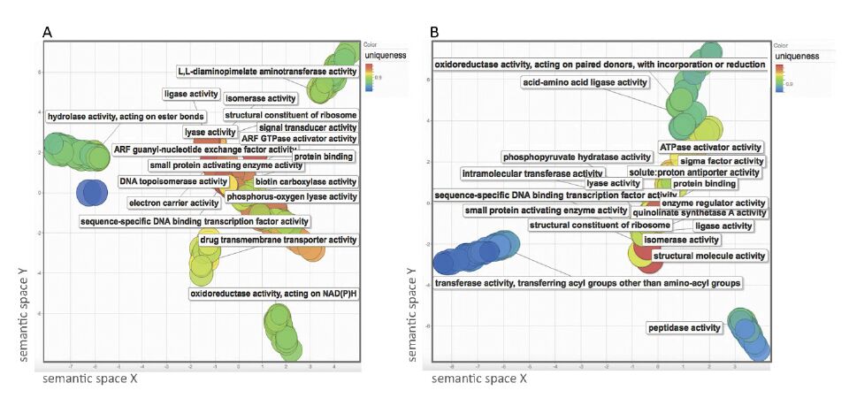
Supek F, Bosnjak M, Skunca N, et al. (2011) REVIGO summarizes and visualizes long lists of gene ontology terms. PLoS One 6: e21800. doi: 10.1371/journal.pone.0021800
  • This article has been cited by:

    1. Teklebirhan Abraha, Fahad Al Basir, Legesse Lemecha Obsu, Delfim F. M. Torres, Farming awareness based optimum interventions for crop pest control, 2021, 18, 1551-0018, 5364, 10.3934/mbe.2021272
    2. Cong Chen, Yibai Li, Guangqiao Cao, Jinlong Zhang, Research on Dynamic Scheduling Model of Plant Protection UAV Based on Levy Simulated Annealing Algorithm, 2023, 15, 2071-1050, 1772, 10.3390/su15031772
    3. Yitian Shao, Jianwei Ni, Shengjia Zhou, Yiping Wang, Xuanxuan Jin, Safety assessment of agricultural products and the pesticide regulation trend in China, 2024, 12, 2193-7532, 10.1186/s40100-024-00322-w
  • Reader Comments
  • © 2015 the Author(s), licensee AIMS Press. This is an open access article distributed under the terms of the Creative Commons Attribution License (http://creativecommons.org/licenses/by/4.0)
通讯作者: 陈斌, bchen63@163.com
  • 1. 

    沈阳化工大学材料科学与工程学院 沈阳 110142

  1. 本站搜索
  2. 百度学术搜索
  3. 万方数据库搜索
  4. CNKI搜索

Metrics

Article views(9525) PDF downloads(1632) Cited by(19)

Figures and Tables

Figures(7)  /  Tables(2)

/

DownLoad:  Full-Size Img  PowerPoint
Return
Return

Catalog