Loading [MathJax]/jax/output/SVG/jax.js
Review

Development of expression systems for the production of recombinant human Fas ligand extracellular domain derivatives using Pichia pastoris and preparation of the conjugates by site-specific chemical modifications: A review

  • Human Fas ligand extracellular domain (hFasLECD) is a biomedically important glycoprotein with three potential N-linked carbohydrate-chain attachment sites. hFasLECD can induce an apoptotic cell-death in many malignant cells. Hence, the creation of novel molecular tools exhibiting useful biological activities, based on the exploitation of this protein domain as their components, opens up a great possibility of the advancements in future medical applications. This review mainly focuses on the development of expression systems for obtaining various derivatives of recombinant hFasLECD using Pichia pastoris and the preparation of the conjugates by site-specific chemical modifications of the expressed products. Firstly, a brief introduction of human Fas ligand protein and an overview of the previous works, on the heterologous expression systems for recombinant hFasLECD as well as the associated derivatives aimed at medical applications, were described. Then, the experimental results, obtained during our investigations into the development of the expression systems for the recombinant hFasLECD derivatives using chemically synthesized artificial genes in Pichia pastoris, were summarized. After that, the current state of the methodology for preparation of the hFasLECD conjugates by site-specific chemical modifications, and the functional characterizations of the prepared conjugates, were presented. Finally, conclusions, including a relevant discussion and future perspectives, are provided.

    Citation: Michiro Muraki. Development of expression systems for the production of recombinant human Fas ligand extracellular domain derivatives using Pichia pastoris and preparation of the conjugates by site-specific chemical modifications: A review[J]. AIMS Bioengineering, 2018, 5(1): 39-62. doi: 10.3934/bioeng.2018.1.39

    Related Papers:

    [1] Zhiyan Ding, Hichem Hajaiej . On a fractional Schrödinger equation in the presence of harmonic potential. Electronic Research Archive, 2021, 29(5): 3449-3469. doi: 10.3934/era.2021047
    [2] Messoud Efendiev, Vitali Vougalter . Linear and nonlinear non-Fredholm operators and their applications. Electronic Research Archive, 2022, 30(2): 515-534. doi: 10.3934/era.2022027
    [3] Bidi Younes, Abderrahmane Beniani, Khaled Zennir, Zayd Hajjej, Hongwei Zhang . Global solution for wave equation involving the fractional Laplacian with logarithmic nonlinearity. Electronic Research Archive, 2024, 32(9): 5268-5286. doi: 10.3934/era.2024243
    [4] Huali Wang, Ping Li . Fractional integral associated with the Schrödinger operators on variable exponent space. Electronic Research Archive, 2023, 31(11): 6833-6843. doi: 10.3934/era.2023345
    [5] Tao Zhang, Tingzhi Cheng . A priori estimates of solutions to nonlinear fractional Laplacian equation. Electronic Research Archive, 2023, 31(2): 1119-1133. doi: 10.3934/era.2023056
    [6] Hui Jian, Min Gong, Meixia Cai . Global existence, blow-up and mass concentration for the inhomogeneous nonlinear Schrödinger equation with inverse-square potential. Electronic Research Archive, 2023, 31(12): 7427-7451. doi: 10.3934/era.2023375
    [7] Xiaoming An, Shuangjie Peng . Multi-peak semiclassical bound states for Fractional Schrödinger Equations with fast decaying potentials. Electronic Research Archive, 2022, 30(2): 585-614. doi: 10.3934/era.2022031
    [8] Shasha Bian, Yitong Pei, Boling Guo . Numerical simulation of a generalized nonlinear derivative Schrödinger equation. Electronic Research Archive, 2022, 30(8): 3130-3152. doi: 10.3934/era.2022159
    [9] Ibtissam Issa, Zayd Hajjej . Stabilization for a degenerate wave equation with drift and potential term with boundary fractional derivative control. Electronic Research Archive, 2024, 32(8): 4926-4953. doi: 10.3934/era.2024227
    [10] Yang Liu, Wenke Li . A family of potential wells for a wave equation. Electronic Research Archive, 2020, 28(2): 807-820. doi: 10.3934/era.2020041
  • Human Fas ligand extracellular domain (hFasLECD) is a biomedically important glycoprotein with three potential N-linked carbohydrate-chain attachment sites. hFasLECD can induce an apoptotic cell-death in many malignant cells. Hence, the creation of novel molecular tools exhibiting useful biological activities, based on the exploitation of this protein domain as their components, opens up a great possibility of the advancements in future medical applications. This review mainly focuses on the development of expression systems for obtaining various derivatives of recombinant hFasLECD using Pichia pastoris and the preparation of the conjugates by site-specific chemical modifications of the expressed products. Firstly, a brief introduction of human Fas ligand protein and an overview of the previous works, on the heterologous expression systems for recombinant hFasLECD as well as the associated derivatives aimed at medical applications, were described. Then, the experimental results, obtained during our investigations into the development of the expression systems for the recombinant hFasLECD derivatives using chemically synthesized artificial genes in Pichia pastoris, were summarized. After that, the current state of the methodology for preparation of the hFasLECD conjugates by site-specific chemical modifications, and the functional characterizations of the prepared conjugates, were presented. Finally, conclusions, including a relevant discussion and future perspectives, are provided.


    In this paper, we examine the following Schrödinger equation:

    $ {iψt=(Δ)sψ+|x|2ψ|ψ|2σψinRN×[0,),ψ(0,x)=ψ0(x)Hs(RN), $ (1)

    where $ 0<s<1 $, $ \sigma>0 $, $ N\geq1 $ and $ \psi: \mathbb{R}^{N}\times [0, \infty)\longrightarrow \mathbb{C} $ is the wave function with initial condition $ \psi_0(x) $ belonging to the following Sobolev space:

    $ Hs(RN):={uL2(RN):RNRN|u(x)u(y)|2|xy|N+2sdydx<}. $

    with

    $ uHs(RN)=RNRN|u(x)u(y)|2|xy|N+2sdydx+RN|u(x)|2dx. $

    The fractional Laplacian $ (-\Delta)^{s} $ is defined via a pseudo-differential operator

    $ (Δ)su(x)=F1[|ξ|2s[u]], s>0. $ (2)

    For the Cauchy problem, formally we have two conserved quantities [17] by multiplying the conjugate of $ \psi $ to both sides and taking the integral: The mass of the wave function:

    $ M(t)=||ψ(,t)||2:=RN|ψ(x,t)|2dxM(0) $ (3)

    and the total energy:

    $ E(t)=RN[Re(ψ(x,t)(Δ)sψ)+|x|2|ψ|21σ+1|ψ(x,t)|2(σ+1)]dxE(0). $ (4)

    In recent years, a great attention has been focused on the study of problems involving the fractional Laplacian, which naturally appears in obstacle problems, phase transition, conservation laws, financial market. Nonlinear fractional Schrödinger equations (FNLS) have been proposed by [20,19,9] in order to expand the Feynman path integral, from the Brownian like to the Lévy like quantum mechanical paths. The stationary solutions of fractional nonlinear Schrödinger equations have also been intensively studied due to their huge importance in nonlinear optics and quantum mechanics [20,19,14,12]. The most interesting solutions have the special form:

    $ ψ(x,t)=eiλtu(x),λR,u(x) isasmoothfunction. $ (5)

    They are called the standing waves. These solutions reduce (1) to a semilinear elliptic equation. In fact, after plugging (5) into (1), we need to solve the following equation

    $ (Δ)su(x)+|x|2u(x)|u(x)|2σu(x)=λu(x)inRN. $ (6)

    The case $ s = 1 $ has been intensively studied by many authors (See [24]). There also exist a considerable amount of results concerning the standing waves and long time behavior of fractional nonlinear Schrödinger equations, we refer the readers to [4,7,6,10,13,16,21,23,22,1] and the references therein.

    In this paper, we mainly focus on the solutions to (6). To the best of our knowledge, our results are new and will open the way to solve other classes of fractional Schrödinger equations. This paper has two main parts: In the first part, we address the existence of standing waves through a particular variational form, whose solutions are called ground state solutions. We prove the existence of ground state solutions (Theorem 2.1), and show some qualitative properties like monotonicity and radiality (Lemma 4). We also show that the ground state solutions are orbitally stable (Def 4.2, Theorem 2.2) if we have the uniqueness of the solutions for the Cauchy problem (1) (Theorem 4.3). We have also addressed the critical case $ \sigma = \frac{2s}{N} $, which is consistent with the case $ s = 1 $ in [11]. The second part of this article deals with the numerical method to solve (1) and the existence of ground state solutions as well as the optimality of our conditions. In this part, we were not only able to show the existence of ground state solutions for $ 0<\sigma<\frac{2s}{N} $ but we also gave a characterizing variational problem ((65)-(66)), which was crucial to find the standing waves for the subcritical $ \frac{2s}{N}\leq\sigma< \frac{2s}{N-2s} $. The numerical results provided a good explanation of the effect of $ s $ on the ground state solution. To reach this goal, we showed that the ground state solution is continuous and decreasing with respect to $ s $ in $ L^2 $ and $ L^\infty $ norm (Figure 3), which is a similar phenomenon to [18]. Besides, like Gross–Pitaevskii equation [11], we examined the convergence property of $ \lambda_c $. It turned out that this convergence property also holds in our case. Second, we checked the stability of ground state solutions for different $ s $. If we add a small perturbation to the initial condition, for different $ s $, the absolute value of the solution will always have periodic behavior, which shows the orbital stability (Figure 7). Furthermore, surprisingly, when $ s $ becomes smaller, the stability is worse, which means the oscillation amplitude in the periodic phenomenon becomes larger (Figure 9, 10a). We then address the case where the harmonic potential is not radial, and we obtained nonradial symmetrical ground state solution (Figure 6a, 6b). Finally, we provided interesting numerical results for the time dynamics of the fractional nonlinear Schrödinger equation (FNLS).

    Figure 3.  Ground state solutions with $ \sigma = 1 $ and different $ s $.
    Figure 6.  Ground state solutions with non-symmetric potential.
    Figure 7.  Energy and stability check with $ s = 0.8 $, $ \sigma = 1 $.
    Figure 9.  Abosolute value of solution with different $ s $.
    Figure 10.  Stability test with $ \psi^s_0(x) = 0.9*u^s_0(x) $.

    The main difficulty of constructing ground state solutions comes from the lack of compactness of the Sobolev embeddings for the unbounded domain $ \mathbb{R}^N $. However, by defining an appropriate function space, in which the norm of the potential is involved, we "recuperate" the compactness (see Lemma 3.1). This fact, combined with rearrangement inequalities is the key point to prove the existence of ground state solutions. In the numerical part, the presence of the harmonic potential term is challenging. One can't take Fourier transform directly on both sides of the equation like [18] because we have the nonlinear term. Unlike in [11], we also can't use finite-difference directly since fractional Laplacian is not a local term. Consequently, we use the splitting method and adopt an idea from [8], where they numerically solve fractional Schrödinger equation without potential energy. By our splitting, we can obtain specific solutions in each small step and also preserve the mass (3). For the ground state solutions, the classical Newton's method [11] is too slow because we have to deal with fractional Laplacian. To overcome this, we borrow an idea from [2] and use normalized gradient flow (NGF) to find the ground state solutions. Moreover, for the case $ \frac{2s}{N}\leq\sigma\leq \frac{2s}{N-2s} $, we have noticed that the energy in the original variational problem can not be bounded from below, therefore, we present a new characterizing variational problem ((65)-(66)) to establish the existence of ground state solutions.

    The paper is organized as follows. In section 2, we give our main results about the existence of ground state solutions and the orbital stability of standing waves. In section 3, we provide proof of existence. Then, in section 4, we discuss the orbital stability. In section 5, we use Split-Step Fourier Spectral method to solve (1) numerically. In section 6, instead of using common iterative Newton's method, we use the NGF method to find ground states when $ 0<\sigma\leq \frac{2s}{N-2s} $. Finally, in section 7, we present our numerical results for the dynamics (1) and compare them with other kinds of Schrödinger equations ([11,18]).

    We use a variational formulation to examine the solution to (6). First, note that if $ \lambda = 0 $, we can find solutions $ u(x) $ to (6) from the critical points of the functional $ \mathcal{J}: H_{s}(\mathbb{R}^{N})\longrightarrow \mathbb{R} $ defined as:

    $ J(u)=12su2L2(RN)+12RN|x|2|u|2dx12σ+2RN|u|2σ+2dx, $ (7)

    where $ \|.\|_{L^2(\mathbb{R}^{N})} $ is the $ L^{2} $-norm and $ \|\nabla_{s}u\|_{L^{2}({\mathbb{R}^{N}})} $ is defined by

    $ \|\nabla_{s}u\|_{L^{2}({\mathbb{R}^{N}})}^{2} = C_{N, s}\int_{\mathbb{R}^{N}}\int_{\mathbb{R}^{N}}\frac{|u(x)-u(y)|^{2}}{|x-y|^{N+2s}}dxdy, $

    with some normalization constant $ C_{N, s} $.

    We can derive (7) by multiplying smooth enough test function $ v(x) $ on both sides of (6) and taking the integral over $ x $. However, instead of directly finding the critical points of (7), we consider a reconstructed variational problem, which can help us find solutions with different $ \lambda $ and any energy. Specifically, for a fixed number $ c>0 $, we need to solve the following constrained minimization problem.

    $ Ic=inf{J(u):uSc}, $ (8)

    with

    $ Sc={uΣs(RN):RN|u|2dx=c2}, $ (9)

    where

    $ Σs(RN)={uHs(RN):uΣs(RN):=u2L2(RN)+su2L2(RN)+xu2L2(RN)<}. $ (10)

    is a Hilbert space, with corresponding natural inner product.

    We claim that for each minimizer $ u(x) $ of the constrained minimization problem (8), there exists some $ \lambda $ such that $ (u(x), \lambda) $ is a solution to (6). To prove the claim, we consider $ \lambda $ as a Lagrange multiplier and define

    $ J(u)=J(u)+λ(u2L2(RN)c2). $ (11)

    The minimizer to problem (8) must be the critical point of (11), satisfying:

    $ J(u)u=0 $ (12)

    and

    $ J(u)λ=0, $ (13)

    where (12) implies (6) and (13) implies (9). In this paper, we will mainly focus on the minimizers of problem (8). The following theorem discusses the existence of such minimizers.

    Theorem 2.1. If $ 0<\sigma<\frac{2s}{N} $, then (8) admits a nonnegative, radial and radially decreasing minimizer.

    Remark 1. There were some works considering standing waves for fractional nonlinear Schrödinger equation with different potential enery and nonlinearity terms. In [6], the authors focus on the case where the nonlinearity term is asymptotically linear with $ \psi\rightarrow \infty $. In [7], the author considers strictly positive potential energy. In our case, the nonlinearity term increases polynomially with $ \psi $ and potential energy is not strictly positive, therefore previous technics can not be applied here directly.

    Remark 2. The condition $ 0<\sigma<\frac{2s}{N} $ is important in our proof for the existence of minimizers. For the critical case $ \sigma = \frac{2s}{N} $, we were able to obtain interesting results (section 7).

    After we construct the ground state solutions, we further investigate their stability. By the definition of (5), the ground state solution moves around a circle when the time changes. Therefore we consider and prove the orbital stability of ground state solution (Def 4.2).

    Theorem 2.2. Suppose that $ 0<\sigma<\frac{2s}{N} $ and (1) has a unique solution with conserved mass (3) and energy (4), then the ground state solutions constructed in Theorem 2.1 are orbitally stable.

    In this section, we will establish the existence of ground state solutions of (6), the main difficulty comes from the lack of compactness of the Sobolev embeddings. Usually, at least when the potential in (1) is radially symmetric and radially increasing, such difficulty is overcome by considering the appropriate function space. More precisely, we have

    Lemma 3.1. Let $ 2\leq p< \frac{2N}{N-2s} $, then the embedding $ \Sigma_{s}({\mathbb{R}^{N}})\subset L^p(\mathbb{R}^N) $ is compact.

    Proof. First, when $ p = 2 $, choose $ R>0 $, then for any $ u(x)\neq 0\in \Sigma_s({\mathbb{R}^{N}}) $, we have

    $ |x|R|u|2dx|R|2|x|R|x|2|u|2dx<|R|2u2Σs(RN) $ (14)

    By the classical Sobolev embedding theorem, for any fixed $ R $, $ H_{s}(|x|<R) $ is compactly embedded in $ L^2(|x|<R) $. Therefore, for any bounded sequence in $ \Sigma_s $, we choose $ R_n>0\rightarrow \infty $. And for each $ n $, we pick out the subsequence that converges in $ L^2(|x|<R_n) $ from former convergence sequence in $ L^2(|x|<R_{n-1}) $. Finally, using the diagonal method combined with (14), we find the convergence sequence in $ L^2(\mathbb{R}^N) $.

    Second, for $ p>2 $, using the fractional Gagliardo-Nirenberg inequality [14], we have

    $ upLp(RN)Ku1θL2(RN)suθL2(RN)Ku1θL2(RN)uθΣs(RN), $ (15)

    for some positive constant $ K $, where $ \theta = \frac{N(p-2)}{2sp}<1 $. Since $ \Sigma_s(\mathbb{R}^N) $ is compactly embedded into $ L^2(\mathbb{R}^N) $, (15) directly implies $ \Sigma_s(\mathbb{R}^N) $ is compactly embedded into $ L^p(\mathbb{R}^N) $ for $ 2\leq p<\frac{2N}{N-2s} $.

    Then we have a lemma showing the existence of $ I_{c} $ and the boundedness of the minimizing sequences.

    Lemma 3.2. If $ 0<\sigma<\frac{2s}{N} $, then $ I_{c}>-\infty $ and all the minimizing sequences of (8) are bounded in $ \Sigma_{s}(\mathbb{R}^{N}) $.

    Proof. First, we prove that $ \mathcal{J}(u) $ is bounded from below. Using the fractional Gagliardo-Nirenberg inequality [14], we certainly have

    $ uL2σ+2(RN)Ku1θL2(RN)suθL2(RN), $ (16)

    for some positive constant $ K $, where $ \theta = \frac{N\sigma}{2s(\sigma+1)}. $

    On the other hand, let $ \epsilon>0 $, and $ p, q>1 $ such that $ \frac{1}{p}+\frac{1}{q} = 1 $, then, using Young's inequality, one gets that

    $ u(2σ+2)(1θ)L2(RN)suθ(2σ+2)L2(RN)1pϵpsupθ(2σ+2)L2(RN)+1qϵquq(1θ)(2σ+2)L2(RN). $ (17)

    Combining (16) and (17), we obtain that for any $ u\in S_{c} $,

    $ RN|u(x)|2σ+2dxϵpK2σ+2psu2L2(RN)+K2σ+2qϵqc2q(1θ)(1+σ), $ (18)

    where $ p = \frac{1}{\theta(1+\sigma)} = \frac{2s}{N\sigma}, \ q = \frac{1}{1-\theta(1+\sigma)} $.

    Hence, from (18) we get:

    $ J(u) $ (19)
    $ =12su2L2(RN)+12RN|x|2|u|2dx12σ+2RN|u|2σ+2dx $ (20)
    $ 12su2L2(RN)+12RN|x|2|u|2dx $ (21)
    $ 12σ+2(ϵpK2σ+2psu2L2(RN)+K2σ+2qϵqc2q(1θ)(1+σ)) $ (22)
    $ (12ϵpK2σ+22p(σ+1))su2L2(RN)+12RN|x|2|u|2dxK2σ+2c2q(1θ)(1+σ)2q(1+σ)ϵq. $ (23)

    Then we choose $ \epsilon $ small enough in (23) to make $ \left(\frac{1}{2}-\frac{\epsilon^{p}K^{2\sigma+2}}{2p(\sigma+1)}\right)>0 $, which implies that $ I_{c}>-\infty $. Finally, for all minimizing sequences $ \{u_n\} $, since $ \mathcal{J}(u_n) $ is bounded from below, $ \{u_n\} $ is bounded in $ \Sigma_{s}(\mathbb{R}^{N}) $ by (23).

    Now, we can use compactness (Lemma 3.1) and boundedness (Lemma 3.2) to prove our existence Theorem 2.1.

    Proof. Let $ \{u_{n}\} $ be a minimizing sequence of (8). By Lemma 3.2, $ \{u_{n}\} $ is bounded in $ \Sigma_{s}(\mathbb{R}^{N}) $. Up to a subsequence, there exists $ u $ such that $ u_{n} $ converges weakly to $ u $ in $ \Sigma_{s}(\mathbb{R}^{N}) $.

    Since $ 2\sigma+2<\frac{2N}{N-2s} $ and $ \Sigma_{s}(\mathbb{R}^{N}) $ is compactly embedded in $ L^{p}(\mathbb{R}^{N}) $ for any $ p $ such that $ 2\leq p<\frac{2N}{N-2s} $, we can further prove that $ u_{n} $ will converge strongly to $ u $ in $ L^2({\mathbb{R}^{N}}) $ and $ L^{2\sigma+2}({\mathbb{R}^{N}}) $ (Lemma 3.1). In particular, $ u_n\rightarrow u $ in $ L^2({\mathbb{R}^{N}}) $, which implies that $ u\in \mathcal{S}_c $.

    On the other hand, thanks to the lower semi-continuity, we have

    $ \|xu\|_{L^2({\mathbb{R}^{N}})}+\|\nabla_{s}u\|_{L^2({\mathbb{R}^{N}})}\leq \liminf\limits_{n\rightarrow \infty} \|\nabla_{s}u_{n}\|_{L^2({\mathbb{R}^{N}})}+\|xu_n\|_{L^2({\mathbb{R}^{N}})}\, . $

    Therefore

    $ IcJ(u)lim infnJ(un)=Ic, $ (24)

    which yields that $ u $ is a minimizer.

    The second step consists of constructing a nonnegative, radial, and radially decreasing minimizer. First, we note that:

    $ s|u|L2(RN)suL2(RN), $ (25)

    which implies that $ \mathcal{J}(|u|)\leq\mathcal{J}(u) $. Using the Schwarz symmetrization [15], we construct a symmetrization function $ u^{\ast} $, which is a radially-decreasing function from $ \mathbb{R}^{N} $ into $ \mathbb{R} $ with the property that

    $ meas\left\{x \in \mathbb{R}^{N}: \left|u(x)\right| > \mu\right\} = meas\left\{x \in \mathbb{R}^{N}: u^{\ast}(x) > \mu\right\}\;{\rm{\;for\;any\;}}\;\mu > 0. $

    It is well-known [15] that

    $ {RN|u|2σ+2dx=RN|u|2σ+2dx,RN|u|2dx=RN|u|2dx,RN|x|2|u|2dxRN|x|2|u|2dx. $ (26)

    Besides, from [3] Lemma 6.3, we also have

    $ suL2(RN)suL2(RN). $ (27)

    Combining (26) and (27), we obtain that

    $ \mathcal{J}(|u|^{\ast})\leq \mathcal{J}(|u|)\leq\mathcal{J}(u), \quad {\rm{for\;any}}\ u\in\Sigma_s(\mathbb{R}^N)\, . $

    Remark 3. By (24) and the weakly convergence, we can also see that:

    $ xuL2(RN)+uL2(RN)+suL2(RN)=limnsunL2(RN)+unL2(RN)+xunL2(RN), $

    which implies that there is a minimizing subseqence $ u_{n_k} $ converging to $ u $ in $ \Sigma_s(\mathbb{R}^N) $.

    Remark 4. If $ u\in\Sigma_s(\mathbb{R}^N) $ is a minimizer to (8), we must have

    $ Ic=J(u)=J(|u|)=J(|u|). $ (28)

    By (27) and (28), we obtain that

    $ suL2(RN)=s|u|L2(RN), $ (29)

    which implies that $ u $ doesn't change sign almost everywhere. Furthermore, we also have

    $ RN|x|2(|u|)2dx=RN|x|2|u|2dx. $ (30)

    which further implies $ |u| = |u|^* $ a.e. by [11]. In conlusion, we obtain a minimizer $ u $ that doesn't change sign and is radially decreasing almost everywhere.

    In this section, we will deal with the orbital stability of the ground state solutions. Let us introduce the appropriate Hilbert space:

    $ ˜Σs(RN):={ω=u+iv:(u,v)Σs(RN)×Σs(RN)}, $

    equipped with the norm $ \|\omega\|^{2}_{\widetilde{\Sigma}_{s}(\mathbb{R}^{N})} = \|u\|^{2}_{\Sigma_{s}(\mathbb{R}^{N})}+\|v\|^{2}_{\Sigma_{s}(\mathbb{R}^{N})} $, which is a Hilbert space.

    In term of the new coordinates, the energy functional reads

    $ ˜J(ω)=12sω2L2(RN)+12RN|x|2|ω(x)|2dx12σ+2RN|ω|2σ+2dx, $

    where $ \|\nabla_s\omega\|_{{L^2({\mathbb{R}^{N}})}}^{2} = \|\nabla_{s}u\|_{{L^2({\mathbb{R}^{N}})}}^{2}+\|\nabla_{s}v\|_{{L^2({\mathbb{R}^{N}})}}^{2} $, we can also prove that $ \widetilde{\mathcal{J}}(\omega) $ remains as a constant with time $ t $ if $ \omega(t, x) $ is a solution to $ (1) $.

    Then, for all $ c>0 $, we set a similar constrained minimization problem

    $ ˜Ic=inf{˜J(ω),ω˜Sc}, $

    where $ \mathcal{\widetilde{S}}_{c} $ is defined by:

    $ ˜Sc={ω˜Σs(RN),RN|ω(x)|2dx=c2}. $

    We also introduce the following sets

    $ Oc={uSc:Ic=J(u)},˜Oc={ω˜Sc:˜Ic=˜J(ω)}. $

    Proceeding as in [4,16], we have the following lemma:

    Lemma 4.1. If $ 0<\sigma<\frac{2s}{N} $, then the following properties hold true:

    (i) The energy functional $ \mathcal{J} $ and $ \widetilde{\mathcal{J}} $ are of class $ C^{1} $ on $ \Sigma_{s}(\mathbb{R}^{N}) $ and $ \widetilde{\Sigma}_{s}(\mathbb{R}^{N}) $ respectively.

    (ii) There exists a constant $ C > 0 $ such that

    $ J(u)Σ1s(RN)C(uΣs(RN)+u2σ+1Σs(RN)),˜J(ω)Σ1s(RN)C(ωΣs(RN)+ω2σ+1Σs(RN)). $

    (iii) All minimizing sequences for $ \widetilde{\mathcal{I}}_{c} $ are bounded in $ \widetilde{\Sigma}_{s}(\mathbb{R}^{N}) $ and all minimizing sequences for $ \mathcal{I}_{c} $ are bounded in $ \Sigma_{s}(\mathbb{R}^{N}) $.

    (iv) The mappings $ c\longmapsto \mathcal{I}_{c}, \, \widetilde{\mathcal{I}}_{c} $ are continuous.

    (v) Any minimizing sequence of $ \mathcal{I}_{c} $, $ \widetilde{\mathcal{I}}_{c} $ are relatively compact in $ \Sigma_{s}(\mathbb{R}^{N}) $, $ \widetilde{\Sigma_{s}}(\mathbb{R}^{N}) $.

    (vi) For any $ c>0 $,

    $ Ic=˜Ic. $

    Proof. (i) We follow the steps of Proposition 2.3 [16] by choosing $ g(x, t) = -t^{\sigma} $. For any $ u, v\in \Sigma_{s}(\mathbb{R}^{N}) $, we can see that the last term of functional

    $ RN|u(x)|2σu(x)v(x)dx $

    is of class $ C^{1} $ on $ \Sigma_{s}(\mathbb{R}^{N}) $. Then by the definition of $ \Sigma_{s}(\mathbb{R}^{N}) $ (see (10)), the first two terms of the functional are of class $ C^1 $ on $ \Sigma_{s}(\mathbb{R}^{N}) $.

    (ii) From (i), $ \mathcal{J} $ is of class $ C^{1} $ on $ \Sigma_{s}(\mathbb{R}^{N}) $. Moreover, for all $ u, v\in \Sigma_{s}(\mathbb{R}^{N}) $, we have

    $ J(u),v=CN,SRNRN|u(x)u(y)||v(x)v(y)||xy|N+2sdxdy+RN|x|2u(x)v(x)dxRN|u(x)|2σu(x)v(x)dx. $

    For the last term, by Hölder's inequality, we have

    $ RN|u(x)|2σu(x)v(x)dxu2σ+1L2σ+2(RN)vL2σ+2(RN). $

    Therefore, there exists $ C>0 $ such that

    $ J(u)Σ1s(RN)C(uΣs(RN)+u2σ+1Σs(RN)). $

    (iii) This is a direct result of Lemma 3.2.

    (iv) Let $ c>0 $ and $ \{c_{n}\}\subset (0, \infty) $ such that $ c_{n}\rightarrow c $. It suffices to prove that $ \mathcal{I}_{c_{n}}\rightarrow \mathcal{I}_{c} $. By the definition of $ \mathcal{I}_{c_{n}} $, for any $ n $, there exists $ u_{n}\in S_{c_{n}} $ such that

    $ IcnJ(un)<Icn+1n. $ (31)

    From (iii), there exists a constant $ C_{1}>0 $ such that for all $ n $, we have

    $ \|u_{n}\|_{\Sigma_{s}(\mathbb{R}^{N})}\leq C_{1}, \;\;\forall\;n\in \mathbb{N}. $

    Setting $ v_{n} = \frac{c}{c_{n}}u_{n} $, then we have that for all $ n\in \mathbb{N} $

    $ vnScandunvnΣs(RN)=|1ccn|unΣs(RN)C1|1ccn|, $

    which implies that

    $ unvnΣs(RN)C1+1fornlargeenough. $ (32)

    We deduce by part (ii) that there exists a positive constant $ K: = K(C_{1}) $ such that

    $ J(u)Σ1s(RN)K,foralluΣs(RN)withuΣs(RN)2C1+1. $ (33)

    By (32) and (33), we get that

    $ |J(vn)J(un)|=|10ddtJ(tvn+(1t)un)dt|supuΣs(RN)2C1+1J(u)Σ1s(RN)vnunΣs(RN)KC1|1ccn|. $ (34)

    Then, from (31) and (34), we obtain that

    $ IcnJ(un)1nJ(vn)KC1|1ccn|1nIcKC1|1ccn|1n $

    Combining this with the fact that $ \lim_{n\rightarrow \infty}c_{n} = c $, it yields

    $ lim infnIcnIc. $ (35)

    Now, from Lemma 3.2 and by the definition of $ \mathcal{I}_{c} $, there exists a positive constant $ C_{2} $ and a sequence $ \{u_{n}\}\subset \mathcal{S}_{c} $ such that

    $ unΣs(RN)C2andlimnJ(un)=Ic. $

    Set $ v_{n} = \frac{c_{n}}{c}u_{n} $, then $ v_{n}\in S_{c_{n}} $, there exists a constant $ L = L(C_{2}) $ such that

    $ \|v_{n}-u_{n}\|_{\Sigma_{s}(\mathbb{R}^{N})}\leq C_{2}\left|1-\frac{c_{n}}{c}\right|\;\;{\rm{and}}\;\;| \mathcal{J}(v_{n})- \mathcal{J}(u_{n})|\leq L\, C_{2}\left|1-\frac{c_{n}}{c}\right|. $

    Combining this with (31), we obtain that

    $ \mathcal{I}_{c_{n}}\leq \mathcal{J}(v_{n})\leq \mathcal{J}(u_{n})+L\, C_{2}\left|1-\frac{c_{n}}{c}\right|. $

    Since $ \lim_{n\rightarrow \infty}c_{n} = c $, we have

    $ lim supnIcnIc. $ (36)

    It follows from (35) and (36) that

    $ \lim\limits_{n\rightarrow \infty}\mathcal{I}_{c_{n}} = \mathcal{I}_{c}. $

    (v) This is a direct result of Remark 3.

    (vi) First, we can see $ \Sigma_s(\mathbb{R}^{N})\subset\widetilde{\Sigma}_s(\mathbb{R}^{N}) $. And for any $ \omega\in\Sigma_s(\mathbb{R}^{N}) $, we have

    $ \widetilde{\mathcal{J}}(\omega) = \mathcal{J}(\omega)\, , $

    which implies that

    $ Ic˜Ic. $ (37)

    Second, for any $ \omega\in\widetilde{\Sigma}_s(\mathbb{R}^N) $, we have

    $ \|\nabla_{s}\omega\|^{2}_{L^2(\mathbb{R}^{N})}\geq\|\nabla_{s}|\omega|\|^{2}_{L^2(\mathbb{R}^{N})}, $

    which implies that

    $ \widetilde{\mathcal{J}}(\omega)\geq \widetilde{\mathcal{J}}(|\omega|) = \mathcal{J}(\omega)\geq \mathcal{I}_c, \quad \forall\omega\in\widetilde{\Sigma}_s(\mathbb{R}^{N}), $

    and

    $ ˜IcIc. $ (38)

    Combining (37) and (38), we finally have $ \widetilde{\mathcal{I}}_c = \mathcal{I}_c. $

    Now, for a fixed $ c > 0 $, we use the following definition of stability (see [5]):

    Definition 4.2 We say that $ \widetilde{\mathcal{O}}_{c} $ is stable if

    $ \widetilde{\mathcal{O}}_{c} $ is not empty.

    ● For all $ \omega_0\in\widetilde{\mathcal{O}}_{c} $ and $ \varepsilon>0, $ there exists $ \delta>0 $ such that for all $ \psi_{0}\in \widetilde{\Sigma}_s(\mathbb{R}^{N}) $, we have

    $ \|\omega_0-\psi_{0}\|_{\widetilde{\Sigma}_{s}(\mathbb{R}^{N})} < \delta\;\Longrightarrow\; \inf\limits_{\omega\in\widetilde{\mathcal{O}}_{c}}\|\omega-\psi\|_{\widetilde{\Sigma}_{s}(\mathbb{R}^{N})} < \varepsilon, $

    where $ \psi $ denotes the solution of (1) corresponding to the initial data $ \psi_{0} $.

    If $ \widetilde{\mathcal{O}}_{c} $ is stable, we say that the ground state solutions in $ \widetilde{\mathcal{O}}_{c} $ are orbitally stable. The following theorem states the orbital stability of $ \widetilde{\mathcal{O}}_c $.

    Theorem 4.3. Suppose that $ 0<\sigma<\frac{2s}{N} $, and (1) with initial data $ \psi_{0} \in\widetilde{\Sigma}_s(\mathbb{R}^{N}) $ has a unique solution $ \psi(t, x)\in \widetilde{\Sigma}_s(\mathbb{R}^{N}) $ with

    $ ψ(t,.)L2(RN)=ψ0(t,.)L2(RN)and˜J(ψ(t,.))=˜J(ψ0(t,.)), $ (39)

    then $ \widetilde{\mathcal{O}}_{c} $ is stable.

    Proof. The proof is by contradiction: Suppose that $ \widetilde{\mathcal{O}}_{c} $ is not stable, then there exists $ \epsilon_{0}>0, \;\omega_0\in\widetilde{\mathcal{O}}_{c} $ and a sequence $ \Phi_{0}^{n}\in \widetilde{\Sigma}_s(\mathbb{R}^{N}) $ such that $ \|\omega_0-\Phi^{n}_{0}\|_{\widetilde{\Sigma}_{s}(\mathbb{R}^{N})}\rightarrow 0\;{\rm{as}}\;n\rightarrow \infty $, but

    $ infZ˜OcΦn(tn,.)Z˜Σs(RN)ε $ (40)

    for some sequence $ \{t_{n}\}\subset \mathbb{R} $, where $ \Phi^{n}(t, .) $ is the unique solution of problem (1) corresponding to the initial condition $ \Phi^{n}_{0} $.

    Let $ \omega_{n} = \Phi^{n}(t_{n}, .) = (u_{n}, v_{n})\in \widetilde{\Sigma}_{s}(\mathbb{R}^{N}) $. Since $ \omega\in\widetilde{\mathcal{S}}_{c} $ and $ \widetilde{\mathcal{J}}(\omega) = \widetilde{\mathcal{I}}_{c} $, it follows from the continuity of $ \|.\|_{L^2(\mathbb{R}^{N})} $ and $ \widetilde{\mathcal{J}} $ in $ \widetilde{\Sigma}_{s}(\mathbb{R}^{N}) $ that

    $ Φn0L2(RN)cand˜J(Φn0)˜Ic, n. $

    Thus, we deduce from (39) that

    $ ωnL2(RN)=Φn0L2(RN)cand˜J(ωn)=˜J(Φn0)˜Ic, n. $ (41)

    Since $ \{\omega_{n}\}\subset \widetilde{\Sigma}_{s}(\mathbb{R}^{N}) $, it is easy to see that $ \{|\omega_{n}|\}\subset \Sigma_{s}(\mathbb{R}^{N}) $. On the other hand, Lemma 4.1 (iii) and the proof of Lemma 3.2 imply that $ \{\omega_{n}\} $ is bounded in $ \widetilde{\Sigma}_{s}(\mathbb{R}^{N}) $. Hence, by passing to a subsequence, there exists $ \omega = (u, v)\in\widetilde{\Sigma}_{s}(\mathbb{R}^{N}) $ such that

    $ unu,vnvandlim infnsunL2(RN)+svnL2(RN)exists. $ (42)

    Now, by a straightforward computation, we obtain that

    $ ˜J(ωn)˜J(|ωn|)=12sωn2L2(RN)12s|ωn|2L2(RN)0, $ (43)

    which implies that

    $ ˜Ic=limn˜J(ωn)lim supnJ(|ωn|). $

    Besides, by (41),

    $ ωn2L2(RN)=|ωn|2L2(RN)=c2nc2. $

    It follows from Lemma 4.1 that we have

    $ lim infnJ(|ωn|)lim infnIcn=Ic. $

    Hence

    $ ˜Ic=limn˜J(ωn)=limnJ(|ωn|)=Ic. $ (44)

    It follows from (42), (43) and (44) that

    $ limnsun2L2(RN)+svn2L2(RN)s(u2n+v2n)122L2(RN)=0, $

    which is equivalent to say that

    $ limnswn2L2(RN)=limns|wn|2L2(RN). $ (45)

    The boundedness of $ \omega_n $ in $ \widetilde{\Sigma_s}(\mathbb{R}^{N}) $ and (45) imply that $ |w_{n}| $ is bounded in $ \Sigma_{s}(\mathbb{R}^{N}) $. Using a similar argument to Lemma 3.1, there exists $ \varphi\in \Sigma_{s}(\mathbb{R}^{N}) $ such that

    $ |ωn|φinΣs(RN)andφL2(RN)=cwithJ(φ)=Ic. $ (46)

    Next, let us prove $ \varphi = |\omega| = \left(|u|^2+|v|^2\right)^{1/2} $. Using (42), it follows that

    $ u_{n}\longrightarrow u\;{\rm{\;and\;}}\;v_{n}\longrightarrow v\;{\rm{\;in\;}}\;L^{2}(B(0, R))\;{\rm{for\;all}}\;R > 0\, . $

    Since $ \left|(u_{n}^{2}+v_{n}^{2})^{\frac{1}{2}}-(u^{2}+v^{2})^{\frac{1}{2}}\right|\leq |u_{n}-u|^{2}+|v_{n}-v|^{2} $, one has

    $ (u_{n}^{2}+v_{n}^{2})^{\frac{1}{2}}\longrightarrow (u^{2}+v^{2})^{\frac{1}{2}}\;\;{\rm{in}}\;\;L^{2}(B(0, R))\, . $

    But $ |\omega_n| = (u_{n}^{2}+v_{n}^{2})^{\frac{1}{2}}\longrightarrow \varphi\;{\rm{in}}\;\Sigma_s(\mathbb{R}^N)\subset L^{2}(\mathbb{R}^N). $ Thus, we certainly have

    $ (u^{2}+v^{2})^{\frac{1}{2}} = |\omega| = \varphi\, . $

    This further implies that

    $ ωL2(RN)=φL2(RN)=c,ωL2σ+2(RN)=φL2σ+2(RN). $ (47)

    and

    $ 12RN|x|2|ω|2dx12σ+2RN|ω|2σ+2dx=12RN|x|2|φ|2dx12σ+2RN|φ|2σ+2dx=limn12RN|x|2|ωn|2dx12σ+2RN|ωn|2σ+2dx. $ (48)

    Additionally, by the lower semi-continuity, we further have

    $ ω2L2(RN)lim infnωn2L2(RN). $ (49)

    Combining (48) with (49) and $ \omega\in\widetilde{\mathcal{S}}_c $, we finally obtain that

    $ ˜Ic˜J(ω)limn˜J(ωn)=˜Ic, $

    which implies that

    $ ω˜Ocandsω2L2(RN)=limnsωn2L2(RN). $ (50)

    Finally, by (46), (47), and (50), we obtain that

    $ ωnωin˜Σs(RN), $

    which contradicts to (40).

    In this section, we consider numerical methods to solve (1) and introduce the Split-Step Fourier Spectral method.

    First, we truncate (1) into a finite computational domain $ [-L, L]^N $ with periodic boundary conditions:

    $ {iψt=(Δ)sψ+|x|2ψ|ψ|2σψ, t>0,ψ(0,x)=ψ0(x), $ (51)

    for $ \textbf{x}\in[-L, L]^N $.

    Let $ \tau>0 $ be the time step, and define the time sequence $ t_n = n\tau $ for $ n\geq0 $ and the mesh size $ h = 2L/J $, where $ J $ is a positive even integer. The spatial grid points are

    $ (xj)n=L+(j)nh, 1nN, $ (52)

    where $ \textbf{j} $ is a $ N $-dimension integer vector with each component between 0 and $ J $.

    Denote $ \psi^n_{\textbf{j}} $ the numerical approximation of the solution $ \psi(\textbf{x}^{\textbf{j}}, t_n) $. By the definition of fractional Laplacian in (2), we use the Fourier spectral method for spatial discretization. Hence, we assume the ansatz:

    $ ψ(xj,t)=kK^ψk(t)exp(iμkxj), $ (53)

    where $ \textbf{K} = \left\{\textbf{k}\in \mathbb{R}^N|-J/2\leq \textbf{k}_l\leq J/2-1, 1\leq l\leq N\right\} $, $ \left(\mu^{\textbf{k}}\right)_k = \textbf{k}_k\pi/L $, $ 1\leq k\leq N $.

    Now, we introduce the Split-step Fourier Spectral method. The main idea of this method is to solve (51) in two splitting steps from $ t = t_n $ to $ t = t_{n+1} $ :

    $ iψt=|x|2ψ|ψ|2σψ, $ (54)
    $ iψt=(Δ)sψ. $ (55)

    First, by multiplying $ \psi^* $ on both sides of (54) and subtracting it from its conjugate, we obtain that $ |\psi(\textbf{x}, t)| = |\psi(\textbf{x}, t_n)| $ for any $ t\in[t_n, t_{n+1}) $. Then (54) can be simplified to

    $ iψt=|x|2ψ|ψ(x,tn)|2σψ. $ (56)

    Second, taking Fourier transform on both sides of (55), we obtain that

    $ id^ψk(t)dt=|μk|2s^ψk(t). $ (57)

    We use the second order Strang splitting method with (56) and (57) as follows:

    $ ψn,1j=ψnjexp(i(|xj|2|ψnj|2σ)τ/2) $ (58)
    $ ψn,2j=kK^ψn,1kexp(i|μk|2sτ)exp(iμkxj) $ (59)
    $ ψn+1j=ψn,2jexp(i(|xj|2|ψn,2j|2σ)τ/2) $ (60)

    where $ \textbf{j} $ comes from (52) and $ n\geq 0 $. For $ n = 0 $, initial condition (51) is discretized as:

    $ ψ0j=ψ0(xj) $ (61)

    This method has spectral order accuracy in space and second order in time. Similar to [8], this method preserves discrete mass corresponding to (3) defined as

    $ Mn=(hNj|ψnj|2)1/2. $ (62)

    To find ground state solutions, we have to solve the following equation corresponding to $ u(x) $:

    $ (Δ)su+|x|2u|u|2σu=λu xRN. $ (63)

    As discussed previously, for $ \sigma<\frac{2s}{N} $, we can solve (8)-(10) to find a solution to (63). In order to calculate the minimizer of $ \mathcal{J}(u) $ in $ S_c $, we use the normalized gradient flow method (NGF) [2]. We first apply the steepest gradient decent method to the energy functional $ \mathcal{J}(u) $ without constraint. Then we project the solution back onto the sphere $ \mathcal{S}_c $ to make sure that the constraint $ ||u||_{L^2(\mathbb{R}^{N})} = c $ is satisfied.

    Thus, for a given sequence of time $ 0 = t_0 < t_1 < ... < t_n $ with fixed time step $ \tau $, we compute the approximated solution $ u^{(n)} $ of the partial differential equation

    $ ut=E(u)u $

    and project it onto $ \mathcal{S}_c $ at each step. Specifically,

    $ {˜ut=(Δ)s˜u|x|2˜u+|˜u|2σ˜u,tn<t<tn+1,˜u(x,tn)=u(n)(x),u(n+1)(x)=c˜u(x,tn+1)||˜u(,tn+1)||L2(RN),. $

    Here, we use semi-implicity time discretization scheme:

    $ {˜u(n+1)˜u(n)Δt=(Δ)s˜u(n+1)|x|2˜u(n+1)+|˜u(n)|2σ˜u(n+1),tn<t<tn+1,˜u(x,tn)=u(n)(x),u(n+1)(x)=c˜u(n+1)(x)||˜u(n+1)()||L2(RN), $

    with

    $ δsxu|j=kK|μk|2sexp(iμkxj) $

    to discretize fractional Laplacian, where $ \textbf{K} $, $ \mu^{\textbf{k}} $ are defined in (53).

    In conlusion, in each step, we solve:

    $ {˜u(n+1)ju(n)jτ=δsx˜u(n+1)|j(|xj|2|u(n)j|2σ)˜u(n+1)ju(n+1)j=c˜u(n+1)jMn, $ (64)

    where $ M^n $ is defined in (62), $ \textbf{j} $ comes from (52) and $ n\geq 0 $. For $ n = 0 $, we guess a starting function and discretize it as (61).

    We need to notice that we can only solve (8) for $ \sigma<\frac{2s}{N} $. If $ \sigma\geq \frac{2s}{N} $, $ \|u\|_{L^{2\sigma+2}(\mathbb{R}^N)} $ can not be bounded by $ \|\cdot\|_{\Sigma_s(\mathbb{R}^N)} $, which causes $ I_c = -\infty $ in $ \mathcal{S}_c $. However, we can use another characterizing variational form and find standing waves to (1) for $ \frac{2s}{N}\leq \sigma<\frac{2s}{N-2s} $.

    For $ \sigma<\frac{2s}{N-2s} $, we define the following constrained minimization problem:

    $ Lc=inf{K(u):uTc} $ (65)

    with

    $ Tc={uΣs(RN):uL2σ+2(RN)=c}, $
    $ K(u)=12su2L2(RN)+12RN|x|2|u(x)|2dx+ω2RN|u(x)|2dx, $ (66)

    where $ \Sigma_s(\mathbb{R}^{N}) $ is defined as (10).

    For $ u\in T_c $, we have the estimate

    $ RN|u(x)|2dx|R|2|x|>R|x|2|u|2dx+|x|<R|u|2dx|R|2|x|>R|x|2|u|2dx+CR,σu2L2σ+2(RN), $

    where $ C_{R, \delta} $ depends on $ R, \delta $. Hence, for $ \omega<0 $, if we choose $ R $ large enough to make $ \left(\frac{1}{2}+\frac{\omega}{R^2}\right)>0 $, we obtain that

    $ K(u)12su2L2+(12+ωR2)RN|x|2|u(x)|2dx+ω2CR,σc2> $ (67)

    for $ u\in T_c $. Besides, if $ \omega>0 $, (67) is greater than $ 0 $. Similar to Lemma 3.2 and Theorem 2.1, there exists a local minimizer for (65) with any $ \omega $ and $ c $.

    Now we see $ \lambda $ as the Lagrange multiplier like (11) but with a different functional

    $ K(u)=K(u)λ2σ+2(u2σ+2L2σ+2(RN)c2σ+2), $

    then the critical points $ u^* $ and $ \lambda^* $ satisfy

    $ (Δ)su+|x|2uλ|u|2σu+ωu=0,xRN $ (68)

    by $ \frac{\partial\mathcal{K}^*(u)}{\partial u} = 0 $. If $ \omega>0 $, by multiplying $ \overline{u^*} $ on both sides of (68) and taking the integral, we can see that:

    $ K(u)=K(u)=λ2c2σ+2>0, $ (69)

    which implies that $ \lambda>0 $. Defining $ u_{\omega, c} = \lambda^{1/2\sigma}u^* $, when $ \omega>0 $, we obtain that

    $ (Δ)suω,c+|x|2uω,c|uω,c|2σuω,c+ωuω,c=0,xRN, $ (70)

    which means $ u_{\omega, c}e^{i\omega t} $ is one standing wave solution to (1). We need to mention that (69), (70) actually showed that we can find a ground state solution by solving (66) if $ L_c = \mathcal{K}(u^*)>0 $. In fact, we have $ \mathcal{K}(u^*)>0 $ with $ \omega<0 $ but not very small. This is related with the smallest eigenvalue of $ \left(-\Delta\right)^s+|x|^2 $ (see detail [11]).

    Now, for $ \frac{2s}{N}\leq\sigma<\frac{2s}{N-2s} $, we use the NGF method and the semi-implicity time discretization scheme to solve the constrained problem (65). Similar to (64), the scheme is

    $ {˜u(n+1)ju(n)jτ=δsx˜u(n+1)|j(|xj|2+u(n)j)˜u(n+1)ju(n+1)j=c˜u(n+1)jMn2σ+2, $ (71)

    where $ M^n_{2\sigma+2} $ is discrete $ L^{2\sigma+2}(\mathbb{R}^N) $ norm

    $ M^n_{2\sigma+2} = \left(h^N\sum\limits_{\textbf{j}}|u^n_{\textbf{j}}|^{2\sigma+2}\right)^{1/(2\sigma+2)} $

    and $ \textbf{j} $ comes from (52) for $ n\geq 0 $. For $ n = 0 $, we guess a starting function and discretize it as (61).

    In this section, we show some numerical results, which can help us understand the ground state solution and also illustrate theoretical results. We have mainly investigated: 1. Ground state solutions with different $ s $. 2. Ground state solutions with non-symmetric potentials. 3. Stability and dynamics.

    First, we solve (8) numerically by (64) in one dimension $ N = 1 $ for the case $ s = 0.8 $ and $ \sigma = 1 $ to obtain a ground state solution $ u_0(x) $. From figure 1a we see that $ u_0(x) $ is radially decreasing as Remark 4.

    Figure 1.  Ground state solution with $ s = 0.8 $, $ \sigma = 1 $, $ L = 10 $ and $ J = 5000 $.

    Second, we use $ u_0(x) $ as initial condition in (1) and investigate time evolution of the standing wave (figure 1b, 2a, 2b). As expected, we see that $ |\psi(x, t)| $ is conserved. And the real and imaginary part of the solution change periodicly with time $ t $.

    Figure 2.  Time dynamics of standing waves with $ s = 0.8 $, $ \sigma = 1 $, $ L = 10 $ and $ J = 5000 $.

    By Theorem 2.1, we can obtain the existence of ground state solutions with $ \sigma<\frac{2s}{N} $. We change $ s $ but keep $ \sigma = 1 $ to obtain ground state solutions with different $ s $. From figure 3a, we can see when $ s $ approaches to $ 0.5 $, ground state solutions become peaked with faster spatial decay. This is a similar result to the case without potential [18]. We also check $ \|\cdot\|_{\Sigma_1(\mathbb{R})} $ of ground state solutions when $ s\rightarrow 0.5 $ in (figure 3b), whose growth shows regularity of the solution becomes worse.

    From figure 3a and figure 3b, it seems ground state solutions change continuously with $ s $. We use $ L^2 $ distance between $ u^s_0(x)-u^1(x) $ to check and see the convergence of ground state solutions in $ L^2 $ space with $ s\rightarrow 1 $ (figure 4).

    Figure 4.  $ L^2 $ distance between ground state solutions of $ s<1 $ and $ s = 1 $ with $ \sigma = 1 $.

    Then, we test another two things. The first is the relationship between the constrained minimal energy in (8) and $ s $. We calculate the discrete energy by

    $ E(s)=hJ1j=0[J/21l=J/2|μl|2s|ˆul|2+|xj|2|uj|21σ+1|uj|2(σ+1)]. $ (72)

    From figure 5a, we find the energy's dependence $ (E(s)) $ on $ s $ is monotonic. When $ s $ approaches to $ 0.5 $, the energy will approach to $ -\infty $ because of the nonlinear term. There are two reasons. First, we keep the $ L^2 $ norm of $ u $ (we test with the same mass $ c $), but the potential term becomes small since $ u $ gathers around $ 0 $. Second, in Lemma 3.2, we need $ \sigma<\frac{2s}{N} $ to bound $ \|u\|_{L^{2\sigma+2}(\mathbb{R}^N)} $, whose boundedness becomes worse when $ s\rightarrow0.5 $. This is different from [18], where they didn't use the variation form and keep the $ L^2 $ norm.

    Figure 5.  Energy and $ \lambda_c $.

    Second, we test the relationship between $ c $ and $ \lambda_c $, where $ c $, $ \lambda_c $ are mass and Lagrange multiplier corresponding to the minimizer (8)-(10). By [11], in the case $ s = 1 $, there exists $ \lambda_0 $ such that for any $ \sigma $,

    $ \lim\limits_{c\rightarrow 0}\lambda_c = \lambda_0\, . $

    We also test this with $ s = 0.8 $. From figure 5b, for different $ \sigma $, when $ c\rightarrow 0 $, $ \lambda_c $ will also converge to a same value $ \lambda_0 $.

    Up to now, we only consider the case with radially symmetrical potential. However, when the potential is not radially symmetric, we can still find a standing wave to (1) using (8). We tried cases where the potential has the form $ |x|^2+a\sin(2\pi x) $ with $ a = 1 $ and $ a = 5 $. From figure 6a and 6b, if we add a nonsymmetrical perturbation to potential, we won't get radially symmetrical ground state solutions.

    First, we consider the case $ s>\frac{N\sigma}{2} $, which is covered by our Theorem 2.2. From the theoretical results and figure 1b, we see that standing waves preserve $ |\psi(x, t)| $ with time $ t $. Therefore, we use $ |\psi(x, t)| $ to draw graphs and test its stability. We consider the case $ s = 0.8 $ and $ \sigma = 1 $. We first test condition (39) in Theorem 2.2 with the initial condition $ \psi_0(x) = (1+e)*u_0(x) $. Because the scheme is mass preserving, it suffices to test energy preservation, which is showed in figure 7a, 7b. Then, we test the stability of the solution, where $ e $ is a constant number. From figure 7c, 7d, when $ e = 0.05 $, the solution almost preserves $ |\psi(x, t)| $ as we desired. When $ e = 0.2 $, the solution shows large perturbation but still has the periodic behavior, similar to [11] and [18]. In figure 8, we compare the $ \|\cdot\|_{\widetilde{\Sigma}_s(\mathbb{R})} $ distance between ground state solutions and perturbed solutions. We can see from figure 3b and theoretical results that when $ s\rightarrow \frac{\sigma N}{2} $, the regularity of ground state solutions becomes worse. This inspires us to investigate its stability relationship with $ s $. By Theorem 2.2, Def 4.2, the orbital stability means we can find $ \omega\in\widetilde{\mathcal{O}}_{c} $ such that $ \|\omega-\psi\|_{\widetilde{\Sigma}_{s}(\mathbb{R})} $ is small when we only have a small perturbation in initial condition. This definition is hard to measure. Instead of checking the exact definition of the orbital stability, we test classical stability by comparing the distance between perturbed solutions and ground state solutions using the normalized $ \|\cdot\|_{\widetilde{\Sigma}_s(\mathbb{R})} $ distance:

    $ D(s, t) = \frac{\|u^s(x, t)-\psi^s(x, t)\|_{\widetilde{\Sigma}_{s}(\mathbb{R})}}{\|u^s(x, t)\|_{\widetilde{\Sigma}_{s}(\mathbb{R})}}. $
    Figure 8.  $ \|\psi^s(x, t)-u^s(x, t)\|_{\widetilde{\Sigma}_s(\mathbb{R})} $ when $ s = 0.8 $ and $ \sigma = 1 $.

    We test initial conditions $ \psi_0(x) = 0.9*u_0(x) $ with $ s = 0.8 $ and $ s = 0.6 $. From figure 9, 10a, as expected, when $ s $ is small, its stability seems worse. To be complete, we test $ D(s, 1) $ with $ s $ between $ 0.51 $ and $ 1 $ in figure 10b. We can see $ D(1, s) $ increases when $ s $ approaches to $ 0.5 $, which implies worse stability.

    Second, we try to obtain some numerical results when we touch the critical point $ s = \frac{\sigma N}{2} $. In this case, we can't find the ground state solution through (8) because $ I_c = -\infty $. However, as we discussed before, we can find a ground state solution related to another constrained minimization problem (65). Here, we try to use the NGF method to find a ground state solution with $ s = 0.5 $, $ \sigma = 1 $. We first tried positive $ \omega $, but the projection step dominated the process (71). Therefore, we tried $ \omega = -0.5 $ and find the method does converge to a solution. From figure 11b-11d, we can see $ |\psi(x, t)| $ is almost preserved with time $ t $ and it has periodical real and imaginary part. We use it to test the finite blowup phenomenon ($ \psi_0(x) = 2u_0(x) $) appeared in the case without potential [18], and this also happens with potential (figure 11e). We note here that we still can't find a perfect ground state solution, which is caused by the stability of (1) is very bad when $ s = 0.5 $.

    Figure 11.  Standing wave, ground state solution and blow up solution with $ s = 0.5 $, $ \delta = 1 $.

    Finally, we test some simple time dynamics of FNLS, we let $ \psi_0(x) = u_0(x)e^{ikx} $, which changes its phase but not absolute value. If $ s = 0.8 $ and $ k = 1, 20 $ (Figure 12a, 12b), the maximum point of $ |\psi(x, t)| $ will move along $ x $ periodically. We also test the $ L^\infty $ norm of $ \psi(x, t) $ (Figure 13a). We find that it decreases first and then approaches to some limits, which is similar to the case without potential [18].

    Figure 12.  Dynamics of FNLS.
    Figure 13.  Evolution of $ L^\infty $.
    [1] Takahashi T, Tanaka M, Inazawa J, et al. (1994) Human Fas ligand: gene structure, chromosomal location and species specificity. Int Immunol 6: 1567–1574. doi: 10.1093/intimm/6.10.1567
    [2] Linkermann A, Qian J, Lettau M, et al. (2005) Considering Fas ligand as a target for therapy. Expert Opin Ther Tar 9: 119–134. doi: 10.1517/14728222.9.1.119
    [3] Yonehara S, Ishii A, Yonehara M (1989) A cell-killing monoclonal antibody (anti-Fas) to a cell surface antigen co-downregulated with the receptor of tumor necrosis factor. J Exp Med 169: 1747–1756. doi: 10.1084/jem.169.5.1747
    [4] Nagata S (1999) Fas ligand-induced apoptosis. Annu Rev Genet 33: 29–55. doi: 10.1146/annurev.genet.33.1.29
    [5] Bodmer JL, Schneider P, Tschopp J (2002) The molecular architecture of the TNF superfamily. Trends Biochem Sci 27: 19–26. doi: 10.1016/S0968-0004(01)01995-8
    [6] Timmer T, de Vries EG, de Jong S (2002) Fas receptor-mediated apoptosis: a clinical application? J Pathol 196: 125–134. doi: 10.1002/path.1028
    [7] Peter ME, Hadji A, Murmann AE (2015) The role of CD95 and CD95 ligand in cancer. Cell Death Differ 22: 549–559. doi: 10.1038/cdd.2015.3
    [8] Calmon-Hamaty F, Audo R, Combe B, et al. (2015) Targeting the Fas/FasL system in rheumatoid arthritis therapy: promising or risky? Cytokine 75: 228–233. doi: 10.1016/j.cyto.2014.10.004
    [9] Wu J, Wilson J, He J, et al. (1996) Fas ligand mutation in a patient with systemic lupus erythematosus and lymphoproliferative disease. J Clin Invest 98: 1107–1113. doi: 10.1172/JCI118892
    [10] Suda T, Takahashi T, Golstein P, et al. (1993) Molecular cloning and expression of the Fas ligand, a novel member of the tumor necrosis factor family. Cell 75: 1169–1178. doi: 10.1016/0092-8674(93)90326-L
    [11] Nagata S (1997) Apoptosis by death factor. Cell 88: 355–365. doi: 10.1016/S0092-8674(00)81874-7
    [12] Wajant H (2006) Fas signaling. New York: Springer Science+Business Media, 1–160.
    [13] Strasser A, Jost PJ, Nagata S (2009) The many roles of Fas receptor signaling in the immune system. Immunity 30: 180–192. doi: 10.1016/j.immuni.2009.01.001
    [14] Bremer E (2013) Targeting of the tumor necrosis factor receptor superfamily for cancer immunotherapy. ISRN Oncol 2013: 371854.
    [15] Hsieh SL, Lin WW (2017) Decoy receptor 3: an endogenous immunomodulator in cancer growth and inflammatory reactions. J Biomed Sci 24: 39. doi: 10.1186/s12929-017-0347-7
    [16] Liu W, Ramagopal U, Cheng H, et al. (2016) Crystal structure of the complex of human FasL and its decoy receptor DcR3. Structure 24: 2016–2023. doi: 10.1016/j.str.2016.09.009
    [17] Muraki M (2012) Heterologous production of death ligands' and death receptors' extracellular domains: structural features and efficient systems. Protein Peptide Lett 19: 867–879. doi: 10.2174/092986612801619606
    [18] Tanaka M, Suda T, Yatomi T, et al. (1997) Lethal effect of recombinant human Fas ligand in mice pretreated with Propionibacterium acnes. J Immunol 158: 2303–2309.
    [19] Muraki M (2006) Secretory expression of synthetic human Fas ligand extracellular domain gene in Pichia pastoris: influences of tag addition and N-glycosylation site deletion, and development of a purification method. Protein Expres Purif 50: 137–146. doi: 10.1016/j.pep.2006.08.006
    [20] Lu Y, Knol JC, Linskens MHK, et al. (2004) Production of the soluble human Fas ligand by Dictyostelium discoideum cultivated on a synthetic medium. J Biotechnol 108: 243–251. doi: 10.1016/j.jbiotec.2003.12.006
    [21] Luo Z, Xu Z, Zhuo S, et al. (2012) Production, purification and cytotoxity of soluble human Fas ligand expressed by Escherichia coli and Dictyostelium discoideum. Biochem Eng J 62: 86–91. doi: 10.1016/j.bej.2012.01.002
    [22] Sun KH, Sun GH, Tsai CY, et al. (2005) Expression, purification, refolding, and characterization of recombinant human soluble-Fas ligand from Escherichia coli. Enzyme Microb Tech 36: 527–534. doi: 10.1016/j.enzmictec.2004.11.013
    [23] Muraki M (2014) Disulfide-bridged proteins with potential for medical applications: therapeutic relevance, sample preparation and structure-function relationships. Integr Mol Med 1: 38–56.
    [24] Holler N, Tardivel A, Kovacsovicsbankowski M, et al. (2003) Two adjacent trimeric Fas ligands are required for Fas signaling and formation of a death-inducing signaling complex. Mol Cell Biol 23: 1428–1440. doi: 10.1128/MCB.23.4.1428-1440.2003
    [25] Eisele G, Roth P, Hasenbach K, et al. (2011) APO010, a synthetic hexameric CD95 ligand, induces human glioma cell death in vitro and in vivo. Neuro-Oncology 13: 155–164. doi: 10.1093/neuonc/noq176
    [26] Eisele G, Wolpert F, Decrey G, et al. (2013) APO010, a synthetic hexameric CD95 ligand, induces death of human glioblastoma stem-like cells. Anticancer Res 33: 3563–3571.
    [27] Oncology venture: APO010, 2012. Available from: http://www.oncologyventure.com/pipeline/apo010/.
    [28] ClinicalTrials.gov: ID NCT03196947, Safety and pharmacokinetics of rising doses of APO010 in relapsed/refractory multiple myeloma patients selected by DRP (SMR-3184). Available from: https://clinicaltrials.gov/ct2/show/NCT03196947?recrs=ab&cond=APO010&rank=1.
    [29] Daburon S, Devaud C, Costet P, et al. (2013) Functional characterization of a chimeric soluble Fas ligand polymer with in vivo anti-tumor activity. Plos One 8: e54000. doi: 10.1371/journal.pone.0054000
    [30] Samel D, Müller D, Gerspach J, et al. (2003) Generation of a FasL-based proapoptotic fusion protein devoid of systemic toxicity due to cell-surface antigen-resticted activation. J Biol Chem 278: 32077–32082. doi: 10.1074/jbc.M304866200
    [31] Bremer E, Ten CB, Samplonius DF, et al. (2008) Superior activity of fusion protein scFvRit:sFasL over cotreatment with rituximab and Fas agonists. Cancer Res 68: 597–604. doi: 10.1158/0008-5472.CAN-07-5171
    [32] Bremer E, Ten CB, Samplonius DF, et al. (2006) CD7-restricted activation of Fas-mediated apoptosis: a novel therapeutic approach for acute T-cell leukemia. Blood 107: 2863–2870. doi: 10.1182/blood-2005-07-2929
    [33] Chien MH, Chang WM, Lee WJ (2017) A Fas ligand (FasL)-fused humanized antibody against tumor-associated glycoprotein 72 selectively exhibits the cytotoxic effect against oral cancer cells with a low FasL/Fas ratio. Mol Cancer Ther 16: 1102–1113. doi: 10.1158/1535-7163.MCT-16-0314
    [34] Chan DV, Sharma R, Ju CYA, et al. (2013) A recombinant scFv-FasLext as a targeting cytotoxic agent against human Jurkat-Ras cancer. J Biomed Sci 20: 16. doi: 10.1186/1423-0127-20-16
    [35] Hemmerle T, Hess C, Venetz D, et al. (2014) Tumor targeting properties of antibody fusion proteins based on different members of the murine tumor necrosis superfamily. J Biotechnol 172: 73–76. doi: 10.1016/j.jbiotec.2013.12.010
    [36] Orbach A, Rachmilewitz J, Shani N, et al. (2010) CD40.FasL and CTLA-4.FasL fusion proteins induce apoptosis in malignant cell lines by dual signaling. Am J Pathol 177: 3159–3168.
    [37] Aronin A, Amsili S, Progozhina T, et al. (2014) Highly efficient in-vivo Fas-mediated apoptosis of B-cell lymphoma by hexameric CTLA4-FasL. J Hematol Oncol 7: 64. doi: 10.1186/s13045-014-0064-6
    [38] Zhang W, Wang B, Wang F, et al. (2012) CTLA4-FasL fusion product suppresses proliferation of fibroblast-like synoviocytes and progression of adjuvant-induced arthritis in rats. Mol Immunol 50: 150–159. doi: 10.1016/j.molimm.2012.01.007
    [39] Shi W, Chen M, Xie L (2007) Prolongation of corneal allograft survival by CTLA4-FasL in a murine model. Graef Arch Clin Exp 245: 1691–1697. doi: 10.1007/s00417-007-0606-5
    [40] Feng YG, Jin YZ, Zhang QY (2005) CTLA4-Fas ligand gene transfer mediated by adenovirus induce long-time survival of murine cardiac allografts. Transpl P 37: 2379–2381. doi: 10.1016/j.transproceed.2005.03.022
    [41] Kitano H, Mamiya A, Kokubun S, et al. (2012) Efficient nonviral gene therapy with FasL and Del1 fragments in mice. J Gene Med 14: 642–650. doi: 10.1002/jgm.2682
    [42] Morello A, Daburon S, Castroviejo M, et al. (2013) Enhancing production and cytotoxic activity of polymeric soluble FasL-based chimeric proteins by concomitant expression of soluble FasL. Plos One 8: e73375. doi: 10.1371/journal.pone.0073375
    [43] Franke DDH, Yolcu ES, Alard P, et al. (2007) A novel multimeric form of FasL modulates the ability of diabetogenic T cells to mediate type 1 diabetes in an adoptive transfer model. Mol Immunol 44: 2884–2892. doi: 10.1016/j.molimm.2007.01.014
    [44] Cereghino JL, Cregg JM (2000) Heterologous protein expression in the methylotrophic yeast Pichia pastoris. FEMS Microbiol Rev 24: 45–66. doi: 10.1111/j.1574-6976.2000.tb00532.x
    [45] Daly R, Hearn MTW (2005) Expression of heterologous proteins in Pichia pastoris: a useful experimental tool in protein engineering and production. J Mol Recogit 18: 119–138. doi: 10.1002/jmr.687
    [46] Ahmad M, Hirtz M, Pichler H, et al. (2014) Protein expression in Pichia pastoris: recent achievements and perspectives for heterologous protein production. Appl Microbiol Biot 98: 5301–5317. doi: 10.1007/s00253-014-5732-5
    [47] 
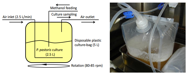
Muraki M (2014) Improved production of recombinant human Fas ligand extracellular domain in Pichia pastoris: yield enhancement using disposable culture-bag and its application to site-specific chemical modifications. BMC Biotechnol 14: 19. doi: 10.1186/1472-6750-14-19
    [48] Jacobs PP, Geysens S, Vervecken W, et al. (2009) Engineering complex-type N-glycosylation in Pichia pastoris using glycoswitch technology. Nat Protoc 4: 58–70. doi: 10.1038/nprot.2008.213
    [49] Helenius A, Aebi M (2004) Roles of N-linked glycans in endoplasmic reticulum. Annu Rev Biochem 73: 1019–1049. doi: 10.1146/annurev.biochem.73.011303.073752
    [50] Pfeffer M, Maurer M, Stadlmann J, et al. (2012) Intracellular interactome of secreted antibody Fab fragment in Pichia pastoris reveals its routes of secretion and degradation. Appl Microbiol Biot 93: 2503–2512. doi: 10.1007/s00253-012-3933-3
    [51] Muraki M (2008) Improved secretion of human Fas ligand extracellular domain by N-terminal part truncation in Pichia pastoris and preparation of the N-linked carbohydrate chain trimmed derivative. Protein Expres Purif 60: 205–213.
    [52] Orlinick JR, Elkon KB, Chao MV (1997) Separate domains of the human Fas ligand dictate self-association and receptor binding. J Biol Chem 51: 32221–32229.
    [53] Gasteiger E, Hoogland C, Gattiker A, et al. (2005) Protein identification and analysis tools on the ExPASy server, In: Walker JM, The Proteomics Protocols Handbook, Totowa: Humana Press, 571–607.
    [54] 
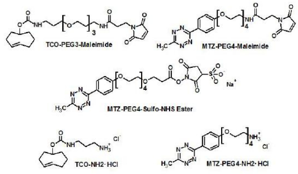
Muraki M, Hirota K (2017) Site-specific chemical conjugation of human Fas ligand extracellular domain using trans-cyclooctene-methyltetrazine reactions. BMC Biotechnol 17: 56. doi: 10.1186/s12896-017-0381-2
    [55] Mahiou J, Abastado JP, Cabanie L, et al. (1998) Soluble FasR ligand-binding domain: high-yield production of active fusion and non-fusion recombinant proteins using the baculovirus/insect cell system. Biochem J 330: 1051–1058. doi: 10.1042/bj3301051
    [56] Muraki M, Honda S (2010) Efficient production of human Fas receptor extracellular domain-human IgG1 heavy chain Fc domain fusion protein using baculovirus/silkworm expression system. Protein Expres Purif 73: 209–216. doi: 10.1016/j.pep.2010.05.007
    [57] Muraki M, Honda S (2011) Improved isolation and purification of functional human Fas receptor extracellular domain using baculovirus-silkworm expression system. Protein Expres Purif 80: 102–109. doi: 10.1016/j.pep.2011.07.002
    [58] Vogl T, Glieder A (2013) Regulation of Pichia pastoris promoters and its consequences for protein production. New Biotechnol 30: 385–404. doi: 10.1016/j.nbt.2012.11.010
    [59] Allais JJ, Louktibi A, Baratti J (1980) Oxidation of methanol by the yeast, Pichia pastoris. Purification and properties of the alcohol oxidase. Agric Biol Chem 44: 2279–2289.
    [60] Muraki M (2014) Secretory production of recombinant proteins in methylotrophic yeast Pichia pastoris using a disposable culture-bag. PSSJ Arch 7: e078.
    [61] Vanamee ÉS, Faustmann DL (2018) Structural principles of tumor necrosis factor superfamily signaling. Sci Signal 11: eaao4910. doi: 10.1126/scisignal.aao4910
    [62] Hermanson GT (2013) Chapter 10: Fluorescent Probes, In: Bioconjugate techniques (Third Ed.), London: Academic Press, 395–463.
    [63] Wu H, Devaraj NK (2016) Inverse electron-demand Diels-Alder biorthogonal reactions. Top Curr Chem 374: 3. doi: 10.1007/s41061-015-0005-z
    [64] Mayer S, Lang K (2017) Tetrazines in inverse-electron-demand Diels-Alder cycloadditions and their use in biology. Synthesis-Stuttgart 49: 830–848.
    [65] Muraki M (2016) Preparation of a functional fluorescent human Fas ligand extracellular domain derivative using a three-dimensional structure guided site-specific fluorochrome conjugation. SpringerPlus 5: 997. doi: 10.1186/s40064-016-2673-8
    [66] Ogasawara J, Watanabe-Fukunaga R, Adachi M, et al. (1993) Lethal effect of the anti-Fas antibody in mice. Nature 364: 806–809. doi: 10.1038/364806a0
    [67] Wajant H, Gerspach J, Pfizenmaier K (2013) Engineering death receptor ligands for cancer therapy. Cancer Lett 332: 163–174. doi: 10.1016/j.canlet.2010.12.019
    [68] Villa-Morales M, Fernández-Piqueras J (2012) Targeting the Fas/FasL signaling pathway in cancer therapy. Expert Opin Ther Tar 16: 85–101. doi: 10.1517/14728222.2011.628937
    [69] Oliveira BL, Guo Z, Bernardes GJL (2017) Inverse electron demand Diels-Alder reactions in chemical biology. Chem Soc Rev 46: 4895–4950. doi: 10.1039/C7CS00184C
    [70] Green NM (1963) Avidin. 4. Stability at extremes of pH and dissociation into sub-units by guanidine hydrochloride. Biochem J 89: 609–620.
    [71] Paganelli G, Magnani P, Zito F, et al. (1991) Three-step monoclonal antibody tumor targeting in carcinoembryonic antigen positive patients. Cancer Res 51: 5960–5966.
    [72] Penichet ML, Kang YS, Pardridge WM, et al. (1999) An antibody-avidin fusion protein specific for the transferrin receptor serves as a delivery vehicle for effective brain targeting: initial applications in anti-HIV antisense drug delivery to brain. J Immunol 163: 4421–4426.
    [73] Schultz J, Lin Y, Sanderson J, et al. (2000) A tetravalent single-chain antibody-streptavidin fusion protein for pretargeted lymphoma therapy. Cancer Res 60: 6663–6669.
    [74] Mohsin H, Jia F, Bryan JN, et al. (2011) Comparison of pretargeted and conventional CC49 radioimmunotherapy using 149Pm, 166Ho, and 177Lu. Bioconjugate Chem 22: 2444–2452. doi: 10.1021/bc200258x
    [75] Micheau O, Solary E, Hammann A, et al. (1997) Sensitization of cancer cells treated with cytotoxic drugs to Fas-mediated cytotoxity. J Natl CancerI 89: 783–789. doi: 10.1093/jnci/89.11.783
    [76] Yang D, Torres CM, Bardhan K, et al. (2012) Decitabine and vorinostat cooperate to sensitize colon carcinoma cells to Fas ligand-induced apoptosis in vitro and tumor suppression in vivo. J Immunol 188: 4441–4449. doi: 10.4049/jimmunol.1103035
    [77] Galenkamp KMO, Carriba P, Urresti J, et al. (2015) TNFα sensitizes neuroblastoma cells to FasL-, cisplatin- and etoposide-induced cell death by NF-ΚB-mediated expression of Fas. Mol Cancer 14: 62. doi: 10.1186/s12943-015-0329-x
    [78] Xu X, Fu XY, Plate J (1998) IFN-γ induces cell growth inhibition by Fas-mediated apoptosis: requirement of STAT1 protein for up-regulation of Fas and FasL expression. Cancer Res 58: 2832–2837.
    [79] Horton JK, Siamakpour-Reihani S, Lee CT, et al. (2015) Fas death receptor: a breast cancer subtype-specific radiation response biomarker and potential therapeutic target. Radiat Res 184: 456–469. doi: 10.1667/RR14089.1
    [80] Tamakoshi A, Nakachi K, Ito Y, et al. (2008) Soluble Fas level and cancer mortality: findings from a nested case-control study within a large-scale prospective study. Int J Cancer 123: 1913–1916. doi: 10.1002/ijc.23731
    [81] Bhatraju PK, Robinson-Cohen C, Mikacenic C, et al. (2017) Circulating levels of soluble Fas (sCD95) are associated with risk for development of a nonresolving acute kidney injury subphenotype. Crit Care 21: 217. doi: 10.1186/s13054-017-1807-x
    [82] Hamilton SR, Gerngross TU (2007) Glycosylation engineering in yeast: the advent of fully humanized yeast. Curr Opin Biotech 18: 387–392. doi: 10.1016/j.copbio.2007.09.001
    [83] Liu L, Stadheim A, Hamuro L, et al. (2011) Pharmacokinetics of IgG1 monoclonal antibodies produced in humanized Pichia pastoris with specific glycoforms: a comparative study with CHO produced materials. Biologicals 39: 205–210. doi: 10.1016/j.biologicals.2011.06.002
  • This article has been cited by:

    1. Mona M. Saber, Nada Monir, Azza S. Awad, Marwa E. Elsherbiny, Hala F. Zaki, TLR9: A friend or a foe, 2022, 307, 00243205, 120874, 10.1016/j.lfs.2022.120874
  • Reader Comments
  • © 2018 the Author(s), licensee AIMS Press. This is an open access article distributed under the terms of the Creative Commons Attribution License (http://creativecommons.org/licenses/by/4.0)
通讯作者: 陈斌, bchen63@163.com
  • 1. 

    沈阳化工大学材料科学与工程学院 沈阳 110142

  1. 本站搜索
  2. 百度学术搜索
  3. 万方数据库搜索
  4. CNKI搜索

Metrics

Article views(6782) PDF downloads(1168) Cited by(2)

Figures and Tables

Figures(8)  /  Tables(1)

Other Articles By Authors

/

DownLoad:  Full-Size Img  PowerPoint
Return
Return

Catalog