
Citation: Michael R Hamblin. Mechanisms and applications of the anti-inflammatory effects of photobiomodulation[J]. AIMS Biophysics, 2017, 4(3): 337-361. doi: 10.3934/biophy.2017.3.337
[1] | Rundong Zhao, Qiming Liu, Huazong Zhang . Dynamical behaviors of a vector-borne diseases model with two time delays on bipartite networks. Mathematical Biosciences and Engineering, 2021, 18(4): 3073-3091. doi: 10.3934/mbe.2021154 |
[2] | Yan-Xia Dang, Zhi-Peng Qiu, Xue-Zhi Li, Maia Martcheva . Global dynamics of a vector-host epidemic model with age of infection. Mathematical Biosciences and Engineering, 2017, 14(5&6): 1159-1186. doi: 10.3934/mbe.2017060 |
[3] | Xia Wang, Yuming Chen . An age-structured vector-borne disease model with horizontal transmission in the host. Mathematical Biosciences and Engineering, 2018, 15(5): 1099-1116. doi: 10.3934/mbe.2018049 |
[4] | Hongyong Zhao, Yangyang Shi, Xuebing Zhang . Dynamic analysis of a malaria reaction-diffusion model with periodic delays and vector bias. Mathematical Biosciences and Engineering, 2022, 19(3): 2538-2574. doi: 10.3934/mbe.2022117 |
[5] | Fahad Al Basir, Yasuhiro Takeuchi, Santanu Ray . Dynamics of a delayed plant disease model with Beddington-DeAngelis disease transmission. Mathematical Biosciences and Engineering, 2021, 18(1): 583-599. doi: 10.3934/mbe.2021032 |
[6] | Rocio Caja Rivera, Shakir Bilal, Edwin Michael . The relation between host competence and vector-feeding preference in a multi-host model: Chagas and Cutaneous Leishmaniasis. Mathematical Biosciences and Engineering, 2020, 17(5): 5561-5583. doi: 10.3934/mbe.2020299 |
[7] | Xinli Hu, Yansheng Liu, Jianhong Wu . Culling structured hosts to eradicate vector-borne diseases. Mathematical Biosciences and Engineering, 2009, 6(2): 301-319. doi: 10.3934/mbe.2009.6.301 |
[8] | Ling Xue, Caterina Scoglio . Network-level reproduction number and extinction threshold for vector-borne diseases. Mathematical Biosciences and Engineering, 2015, 12(3): 565-584. doi: 10.3934/mbe.2015.12.565 |
[9] | Hai-Feng Huo, Fan Wu, Hong Xiang . On threshold dynamics for periodic and time-delayed impulsive systems and application to a periodic disease model. Mathematical Biosciences and Engineering, 2022, 19(1): 836-854. doi: 10.3934/mbe.2022038 |
[10] | Lin Zhao, Zhi-Cheng Wang, Liang Zhang . Threshold dynamics of a time periodic and two–group epidemic model with distributed delay. Mathematical Biosciences and Engineering, 2017, 14(5&6): 1535-1563. doi: 10.3934/mbe.2017080 |
Vector-borne disease involves a vector (an organism) that transmits infectious pathogens from the infected host to the uninfected host. For example, the malaria parasites are transmitted through the bite of infected female mosquitoes, spreading the disease from mosquitoes to humans and back to mosquitoes [2]. West Nile virus (WNv) is another vector-borne disease caused by Flavivirus and transmitted primarily by mosquitoes (Culex species) to vertebrate hosts, such as humans, birds and horses [3]. Those vector-borne diseases have caused a significant threat to public health as well as wildlife worldwide.
Mathematical models give insights to predict the spread of vector-borne diseases, and to test control strategies. Impulsive (delayed) differential systems are widely used in population biology and epidemiology to study the various factors: birth pulses [4,5], effectiveness of vaccination [6,7,8,9,10], and elimination of vector insects [11,12], see also [13,14] for stochastic effects. To investigate the control strategies against vector-borne diseases, Gourley et al. [11] used two time-delayed models with impulses to evaluate the effectiveness of age-structured culling strategies. Yang et al. [10] studied the effect of impulsive controls in multiple patch models with age-structure. Xu and Xiao [9] considered the impacts of periodic impulsive culling of mosquitoes for control of WNv transmission. Based on [9], the incubation period of mosquitoes was furthered incorporated in [15].
To describe the disease transmission between vector and host as well as the strategy of periodically culling the vector, we use a set of impulsive delayed differential equations to incorporate the extrinsic incubation period (EIP) of vector and host. By the theory recently developed in [1], the basic reproduction ratio R0 of the model is first established. The global dynamics of the model are further investigated in terms of R0. The uniform persistence theory based on dynamical systems is used extensively in population biology and epidemiology models, see for instance [16,17,18,19] and references therein. However, it seems like this dynamical system approach is rarely adapted to time-delayed impulsive systems to study the threshold dynamics. There are two possible issues: first, it is not an easy task to find an appropriate phase space for time-delayed impulsive systems so that the evolution operators are well-defined, which was recently solved by [1] for a large class of time-delayed impulsive systems; second, the solutions of the time-delayed impulsive systems may not be continuous in t, and hence, such systems might not generate continuous periodic semiflows (see [20]), which brings trouble for direct application of the uniform persistence theory in [21] to investigate the sharp permanence of infectious compartments when R0>1. Meanwhile, the analytic method developed in [1,6,7] for the uniform persistence of a time-delayed impulsive system is quite useful for a form like Susceptible-Exposed-Infected-Removed (SEIR), but it would not be easy to apply to the vector-borne model (including multiple infected compartments). We refer to [9,15] for attempts in this direction. Combing the ideas in [1] and [21], we establish the sharp persistence of infectious compartments, by using the uniform persistence theory of discrete-time semiflows on some appropriate phase space. It is worth pointing out that our current approach would be easily applied to the models where the period of model coefficients is the same as that of fixed impulsive moments.
The rest of this paper is organized as follows: In Section 2, we formulate a time-delayed impulsive differential model including several factors: EIP and the strategy of periodically culling the vector, EIP and vertical transmission of host. In Section 3, we first introduce the basic reproduction number R0 for the model and then study the threshold dynamics in terms of R0. In Section 4, we use numerical simulations to test the differences with and without culling, and further explore the impacts of parameters such as time delays and vertical transmission rate on R0. A brief discussion then concludes the paper.
Inspired by the WNv infection process in [9,15,18], we consider an impulsive delay differential equation model to describe the periodic culling of the vector with two differnt EIPs. Let Sv(t), Iv(t), Sh(t), Eh(t) and Ih(t) be the the total numbers of the susceptible adult vector, infected adult vector, susceptible host, exposed host and infected host at time t, respectively. The total number of the adult vector is given by Nh(t)=Sh(t)+Eh(t)+Ih(t). Let Λv and Λh be the recruitment rate of the vector and (susceptible) host, respectively, μv and μh be the natural death rate of vector and host, and dh be the disease-induced death rate of the host. Similar to [7], we suppose that the birth rate of the vector equals its natural death rate. Vertical transmission of the virus in the host population is incorporated by a fraction rvt∈(0,1). For the virus transmission, we assume that the susceptible host becomes infectious given contact with the infected vector, and the susceptible vector can receive the infection by biting a virus-carrying host. By similar arguments to those in [2,17,19], we simply assume that the numbers of newly occurred infectious host and newly occurred infected vector per unit time at time t are given by
bβIh(t)Nh(t)Sv(t) and cβSh(t)Nh(t)Iv(t), |
respectively, where β is the average biting rate of the vector, b and c are the transmission probabilities of the virus from vector to host and from host to vector, respectively. However, the newly infected vector and infected host need to survive the EIP to become infectious. We denote the finite constants τ1 and τ2 to represent the length of the EIP in the vector and host, respectively. The probability that the vector and host survive the EIP is e−μvτ1 and e−μhτ2, then of those vectors and hosts infected τ1 and τ2 unit times ago, only the proportions
bβIh(t−τ1)Nh(t−τ1)Sv(t−τ1)e−μvτ1 and cβSh(t−τ2)Nh(t−τ2)Iv(t−τ2)e−μhτ2 |
are infectious at time t. Throughout this paper, we suppose that culling occurs at certain particular times, and denote T to be the period of culling. We also assume that spraying reduces both the susceptible and infected vector, p∈[0,+∞) is the culling intensity of those killed, where p=0 means that there is no culling.
The transmission of cross-infection between vector and host is shown in Figure 1. Consequently, our model takes the form:
{dSv(t)dt=Λv−bβIh(t)Nh(t)Sv(t)−μvSv(t),dIv(t)dt=bβIh(t−τ1)Nh(t−τ1)Sv(t−τ1)e−μvτ1−μvIv(t),dSh(t)dt=Λh−cβSh(t)Nh(t)Ih(t)−μhSh(t)+(1−rvt)μhIh(t),dEh(t)dt=cβSh(t)Nh(t)Ih(t)−cβSh(t−τ2)Nh(t−τ2)Iv(t−τ2)e−μhτ2−μhEh(t),dIh(t)dt=cβSh(t−τ2)Nh(t−τ2)Iv(t−τ2)e−μhτ2−(μh+dh−rvtμh)Ih(t),}a.e.t≠nT,n∈N,Sv(t+)=11+pSv(t),Iv(t+)=11+pIv(t),Sh(t+)=Sh(t),Eh(t+)=Eh(t),Ih(t+)=Ih(t),}t=nT,n∈N. | (2.1) |
All the parameters in model (2.1) are positive. In view of the biological meaning of τ2, we impose the following compatibility condition:
ϕ4(0)=∫0−τ2cβϕ2(s)ϕ3(s)∑5i=3ϕi(s)eμhsds. | (2.2) |
To investigate the long time behavior of system (2.1) from the point view of dynamical systems, we first introduce a few notations related to the phase space (see also [1,22]). Given two constants a<b, let
PC([a,b],Rm):={ϕ:[a,b]→Rm|ϕ(t−)=ϕ(t),∀t∈(a,b],ϕ(t+) exists for t∈[a,b) and ϕ(t+)=ϕ(t) for all but at most a finite number of points t∈[a,b)},PC([a,b),Rm):={ϕ:[a,b)→Rm|ϕ(t−)=ϕ(t),∀t∈(a,b),ϕ(t+) exists for t∈[a,b) and ϕ(t+)=ϕ(t) for all but at most a finite number of points t∈[a,b)}, |
where ϕ(t+)=lims→t+ϕ(s) and ϕ(t−)=lims→t−ϕ(s). Then for any r>0, PC([−r,0],Rm) is a Banach space with the norm ‖⋅‖r given by ‖ϕ‖r=sup−r≤θ≤0|ϕ(θ)|. Set ˆτ=max{τ1,τ2}>0, ˜J=[−ˆτ,0)∩{tn=nT:n∈Z}(possibly empty) and J=[−ˆτ,0)∖˜J. Denote
PCJ:={ϕ:[−ˆτ,0]→R|ϕ(t−)=ϕ(t),∀t∈(−ˆτ,0],ϕ(t+) exists for t∈[−ˆτ,0) and ϕ(t+)=ϕ(t) for t∈J}, |
and PC+J:={ϕ∈PCJ:ϕ(t)≥0,∀t∈[−ˆτ,0]}. It then follows that PCJ is a Banach space endowed with the norm ‖⋅‖ˆτ, and PC+J is a closed cone of PCJ, which induces a partial ordering on PCJ. Clearly, PCJ⊂PC([−ˆτ,0],R). For any u=(u1,u2,...,u5)∈PC([−ˆτ,η),R5) with η>0, define ut∈PC([−ˆτ,0],R5) by
ut(θ)=(u1(t+θ),u2(t+θ),...,u5(t+θ)),∀θ∈[−ˆτ,0],t∈[0,η). |
Define
X:={ϕ=(ϕ1,ϕ2,...,ϕ5)∈PC+J×PC+J×PC+J×PC+J×PC+J:5∑i=3ϕi(θ)>0,θ∈[−ˆτ,0]}, |
and
Dϵ:={ϕ∈X:5∑i=3ϕi(θ)>ϵ,∀θ∈[−ˆτ,0],ϕ4(0)=∫0−τ2cβϕ2(s)ϕ3(s)∑5i=3ϕi(s)eμhsds} | (2.3) |
for any ϵ∈(0,Λhμh+dh). Now we are ready to state the well-posed result on the solutions of system (2.1).
Theorem 2.1. For any ϕ∈Dϵ, system (2.1) exists a unique non-negative solution u(t,ϕ) on [0,+∞) with the initial value u0=ϕ, unT∈Dϵ for any n∈N. Moreover, ut+T(ϕ)=ut(uT(ϕ)) for all t≥0 and Φ:=uT admits a global attractor in Dϵ.
Proof. For convenience, we denote
(u1(t),u2(t),u3(t),u4(t),u5(t))=(Sv(t),Iv(t),Sh(t),Eh(t),Ih(t)). |
For any t≥0,t≠nT,n∈N,ϕ∈Dϵ, define
f(t,ϕ):=(f1(ϕ),f2(ϕ),f3(ϕ),f4(ϕ),f5(ϕ)), |
where
f1(ϕ)=Λv−bβϕ5(0)∑5i=3ϕi(0)ϕ1(0)−μvϕ1(0),f2(ϕ)=bβϕ5(−τ1)∑5i=3ϕi(−τ1)ϕ1(−τ1)e−μvτ1−μvϕ2(0),f3(ϕ)=Λh−cβϕ3(0)∑5i=3ϕi(0)ϕ3(0)−μhϕ5(0)+(1−rvt)μhϕ5(0),f4(ϕ)=cβϕ3(0)∑5i=3ϕi(0)ϕ5(0)−cβϕ3(−τ2)∑5i=3ϕi(−τ2)ϕ5(−τ2)e−μhτ2−μhϕ4(0),f5(ϕ)=cβϕ3(−τ2)∑5i=3ϕi(−τ2)ϕ5(−τ2)e−μhτ2−(μh+dh−rvtμh)ϕ5(0). |
It is easy to check that f(t,ϕ) satisfies Lipschitz condition for ϕ on any compact subset of R+×X. It follows from [22, Theorems 3.1 and 3.3] that system (2.1) admits a unique solution u(t,ϕ) satisfying ∑5i=3ui(t,ϕ)>ϵ on the maximal existence interval [0,tϕ) with u0=ϕ∈Dϵ and tϕ∈(0,∞).
Next we prove the solution of system (2.1) is non-negative on [0,tϕ). Given ϕ∈Dϵ and t∈[0,T), we see that fi(t,ϕ):=fi(ϕ)≥0 provided i∈{1,2,3,5} and ϕi(0)=0. It follows from [23, Theorem 5.2.1] and its proof that for ui(t,ϕ)≥0,i∈{1,2,3,5}, ∀t∈[0,T)∩[0,tϕ). If T<tϕ, then by the formulas of system (2.1) at the impulsive points, we have ui(t,ϕ)≥0,i∈{1,2,3,5},t∈[0,T]. It then follows from the method of steps that ui(t,ϕ)≥0,i∈{1,2,3,5},t∈[0,tϕ). Meanwhile, by the uniqueness of solutions of system (2.1) and the compatibility condition (2.2), we obtain that
u4(t)=∫tt−τ2cβu2(s)u3(s)∑5i=3ui(s)e−μh(t−s)ds. | (2.4) |
Therefore, u4(t,ϕ)≥0 for t∈[0,tϕ).
Notice that the total host population (Nh(t):=∑5i=3ui(t)) satisfies
dNh(t)dt=Λh−μhNh(t)−(dh−μh)Ih(t)≥Λh−(μh+dh)Nh(t), | (2.5) |
which implies Nh(t) is an upper solution of
x′(t)=Λh−(μh+dh)x(t). | (2.6) |
Denote x(t;Nh(0)) as the unique solution of (2.6) with x(0)=Nh(0), then Nh(t)≥x(t;Nh(0)) for any t∈[0,tϕ). This further yields that Nh(t)≥x(t;Nh(0))≥ϵ for any t∈[0,tϕ) provided Nh(0)≥ϵ with ϵ∈(0,Λhμh+dh). Furthermore,
dNh(t)dt≤Λh−min{μh,dh}Nh(t), | (2.7) |
which implies that if ϵ≤∑5i=3ϕi(0)≤Λhmin{μh,dh}, then ϵ≤∑5i=3ui(t)≤Λhmin{μh,dh} for any t∈[0,tϕ).
Since ϵ≤Nh(t) and u5(t)≤Nh(t) for any t∈[0,tϕ), by comparison, we have
u′1(t)≤Λv−μvu1,t>0,u′2(t)≤bβu1(t−τ1)e−μvτ1−μvu2,t>0, |
which yields that,
lim supt→∞u1(t)≤Λvμv,lim supt→∞u2(t)≤bβΛve−μvτ1μ2v and lim supt→∞Nh(t)≤Λhmin{μh,dh}. |
Therefore, the solutions of system (2.1) with initial data in Dϵ exist globally on [0,∞) and are ultimately bounded. By similar argument to that in [1, Lemma 4] (see also [24, Page 192]), we infer that for each n>ˆτT, unT is compact. It then follows from [21, Theorem 1.1.3] that UT:Dϵ→Dϵ admits a global attractor. Moreover, since if ut(ϕ) is a solution of (2.1), then ut+T(ϕ) is also a solution (2.1). By the uniqueness of the solution, we then have ut+T(ϕ)=ut(uT(ϕ)).
In this section, we first introduce the basic reproduction number R0 for system (2.1) and then investigate its threshold dynamics in terms of R0.
The basic reproduction number R0 is defined as the expected number of secondary infections produced by a typical infectious individual in a completely susceptible population. We will use the theory developed in [1] to give the definition of R0. In order to obtain the disease-free periodic solution of system (2.1), we recall a lemma (see [6, Lemma 1] for detail).
Lemma 3.1. Consider the following impulsive differential equation:
{dudt=a−bu(t),t≠nT,n∈N,u(t+)=(1−θ)u(t),t=nT,n∈N, | (3.1) |
where a,b>0, θ∈(0,1). Then system (3.1) admits a unique positive periodic solution ˆue(t):=ab+(u∗−ab)e−b(t−nT), nT<t<(n+1)T, which is globally asymptotically stable. Here u∗=a(1−θ)(1−e−bT)b(1−(1−θ)e−bT).
Letting Iv=Ih=0 in system (2.1), we then get the following disease-free system:
{dSv(t)dt=Λv−μvSv(t),dSh(t)dt=Λh−μhSh(t),}a.e.t≠nT,n∈N,Sv(t+)=11+pSv(t),Sh(t+)=Sh(t),}t=nT,n∈N. | (3.2) |
By Lemma 3.1, system (3.2) exists a unique positive T-periodic solution ˆu(t):=(ˆSv(t),ˆSh), with ˆSh=Λhμh and
ˆSv(t)=(1−pe−μv(t−nT)1+p−e−μvT)Λvμv,nT<t≤(n+1)T,n∈N, | (3.3) |
which is globally asymptotically stable.
Let E=PC([−ˆτ,0],R2), E+={ϕ∈E:ϕ(t)≥0,t∈[−ˆτ,0]}, and
XT={v:R→R2|v is continuous in (tn,tn+1),tn=nT,n∈Z,v(t−n),v(t+n) exist v(t−n)=v(tn),v(t+T)=v(t) for t∈R, and v(t+n+1)=v(t+n)}, |
with the norm ‖v‖XT=supt∈[0,T]|v(t)|. It then follows that XT is a Banach space. Linearizing system (2.1) at its disease-free periodic solution E0(t)=(ˆSv(t),0,ˆSh(t),0,0), we obtain the following linear system for the infectious compartments:
{dIv(t)dt=−μvIv(t)+bβe−μvτ1μhΛhˆSv(t−τ1)Ih(t−τ1),dIh(t)dt=−(μh+dh−rvtμh)Ih(t)+cβe−μhτ2Iv(t−τ2),}t≠nT,n∈N,Iv(t+)=11+pIv(t),Ih(t+)=Ih(t),}t=nT,n∈N. | (3.4) |
Define F(t):E→R2, where
F(t)(ϕ1ϕ2):=(bβe−μvτ1μhΛhˆSv(t−τ1)ϕ2(−τ1)cβe−μhτ2ϕ1(−τ2)+rvtμhϕ2(0)),∀t∈R,ϕ=(ϕ1,ϕ2)∈E. |
Set Y(t,s),t≥s as the Cauchy matrix [24, Section 1.2] of
{du1(t)dt=−μvu1(t),du2(t)dt=−(μh+dh)u2(t),}t≠nT,n∈N,u1(t+)=11+pu1(t),u2(t+)=u2(t),}t=nT,n∈N, | (3.5) |
that is,
Y(t,s)=e−V(t−s)∏k:tk∈[s,t)diag (11+p,1), |
where each tk denotes the impulsive point on [s,t) and V=(μv00μh+dh). It is easy to check that F(t) and Y(t,s) satisfy the following properties: (a) for each t∈R, F(t) is a positive operator; (b) the matrix −V is cooperative and r(Y(T,0))<1, where r(Y(T,0) is the spectral radius of Y(T,0).
Consequently, the linear impulse periodic differential system (3.5) could be rewritten as:
{du(t)dt=F(t)ut−Vu(t), a.e. t>0,t≠tn,u(t+)=Pu(t),t=tn,n∈N, | (3.6) |
where P= diag (11+p,1).
After the above settings, we can apply the theory and method in [1] to define basic the reproduction number for system (2.1). Let v(t) be the initial distribution of infected individuals with period T. For t≥s, then F(t−s)vt−s is the distribution of newly infected individuals at time t−s. It is produced by infected individuals introduced during the time interval [t−s−ˆτ,t−s], which means it is the distribution of newly infected at time t−s and still infected at time t. Define the linear operator L on XT:
[Lv](t):=∫∞0Y(t,t−s)F(t−s)v(t−s+⋅)ds,t∈R,∀v∈XT. |
We define the basic reproduction number as
R0:=r(L), |
where r(L) is the spectral radius of the linear operator L. Denote
EJ=PCJ×PCJ,E+J=PC+J×PC+J. |
For any ϕ∈EJ, let w(t,ϕ)=(w1(t,ϕ),w2(t,ϕ)) be the unique solution of (3.4) with the initial value w0=ϕ, and
wt(ϕ)(θ)=(w1t(ϕ)(θ),w2t(ϕ)(θ))=(w1(t+θ,ϕ),w2(t+θ,ϕ)),∀θ∈[−ˆτ,0]. |
Let Q(t):EJ→E=PC([−ˆτ,0],R2) be the solution map of (3.4), then
Q(t)ϕ=(w1t(ϕ),w2t(ϕ)),∀t≥0,ϕ∈EJ. |
In view of the definition of PCJ, we infer that Q:=Q(T) is the operator from EJ to EJ (in other words, they have the same number of discontinuous points), and set r(Q) to be the spectral radius of Q on EJ. By [1, Theorem 1], we have the following observation:
Lemma 3.2. R0−1 has the same sign as r(Q)−1.
Let
Z:=PCτ2×PCτ1,Z+:=PC+τ2×PC+τ1, |
where PCτi is understood as PCJ with ˆτ replaced by τi, and then (Z,Z+) is an ordered Banach space. For any ψ∈Z+, system (3.4) admits a unique non-negative solution z(t,ψ) with the intial value z0=ψ. For all t≥0, we have zt(ψ)=(z1t(ψ),Z2t(ψ)), for all θi∈[−τi,0], and then Zit(ψ)(θi)=zi(t+θi,ψ), i=1,2. For any given t≥0, let ˆQ(t) be the solution map of system (3.4) on Z, that is,
ˆQ(t)ψ=zt(ψ),∀ψ∈Z. |
We remark that z1t∈PC([−τ2,0],R) and z2t∈PCτ1 for all t≥0 as z2(t,ψ) is continuous for all t≥0 even if ψ is piecewise continuous. Therefore, ˆQ(T) is a map from Z to Z. Next, we will illustrate that ˆQ(t) is eventually strongly positive on Z+.
Lemma 3.3. ˆQ(t)φ≫0 for any t>3ˆτ provided φ=(φ1,φ2)∈Z+∖{0}.
Proof. For convenience, denote
(z1(t),z2(t)):=(z1(t,φ),z2(t,φ)). |
By the similar argument to that in Theorem 2.1, we obtain that zi(t)≥0 for any t≥0, i=1,2.
In the case that φ1>0. We argue that there exists ˆt∈[0,ˆτ] such that z2(ˆt)>0. Assume, by contradiction, that z2(t)=0 for all t∈[0,ˆτ], that is, z′2(t)=0 for all t∈[0,ˆτ]. Then we deduce from the second equation of system (3.4) that:
z1(t−τ2)=0,∀t∈[0,ˆτ]. |
This yields φ1(t)≡0 for any t∈[−τ2,0], which is a contradiction. Moreover, from the second equation of system (3.4) and z1(t)≥0 for all t≥−τ2, we obtain
z2(t)≥z2(ˆt)e−(μh+dh−rvtμh)(t−ˆt)>0 for all t≥ˆt. |
Then by the integral form of the first equation of system (3.4), we have
z1(t)=T(t,0)z1(0)+bβe−μvτ1μhΛh∫t0T(t,s)ˆSv(s−τ1)z2(s−τ1)ds, |
where
T(t,s)=e−μv(t−s)∏k:kT∈[s,t)11+p. |
Since ˆt∈[0,ˆτ], it follows that z1(t)>0 for all t>2ˆτ. The result as follows.
In the case that φ2>0. We have
z1(t)≥bβe−μvτ1μhΛh∫t0T(t,s)ˆSv(s−τ1)z2(s−τ1)ds>0 |
provided t>ˆτ. Then by the integral form of the second equation of system (3.4), we have
z2(t)=e−(μh+db−rvtμh)tz2(0)+cβe−μhτ2∫t0e−(μh+dh−rvtμh)(t−s)z1(s−τ2)ds,≥cβe−μhτ2∫t0e−(μh+db−rvtμh)(t−s)z1(s−τ2)ds>0, |
whenever t≥2ˆτ. Therefore, ˆQ(t)φ≫0 for t>3ˆτ.
Denote r(ˆQ) as the spectral radius of ˆQ:=ˆQ(T). One might perform the same argument as in [16, Lemma 3.8] to obtain r(Q)=r(ˆQ). Moreover, we have the following observation:
Lemma 3.4. Let μ=lnr(Q)T. Then there exists a positive T-periodic function ˜v(t)=(˜v1(t),˜v2(t)) such that eμtˆv(t) is a solution of system (3.4) with the feasible domain either Z+ or E+J for any t≥0.
Proof. Resembling the arguments in [1, Lemma 4], we infer that for each t>ˆτ, Q(t) and ˆQ(t) are compact on EJ and Z, respectively.
In the case that the feasible domain is Z+, fix an integer n0>0 such that n0T>3ˆτ. It follows that ˆQn0=ˆQ(n0T) is compact and strongly positively on Z. By [25, Lemma 3.1], we obtain that there is a strongly positive eigenvector φ∗=(φ∗1,φ∗2) such that ˆQ(φ∗)=r(ˆQ)φ∗. Let v(t,φ∗) be the solution of system (3.4) with the initial value
(v1(θ1),v2(θ2))=(φ∗1(θ1),φ∗2(θ2)),(θ1,θ2)×[−τ2,0]×[−τ1,0]. |
Since φ∗≫0, it is easy to see that vt(φ∗)≫0 for any t≥0. Let ˆv(t)=e−μtv(t,φ∗). Then ˆv(t)≫0 satisfies
{dˆv1(t)dt=−μvˆv1(t)+bβe−μvτ1μhΛhˆSv(t−τ1)ˆv2(t−τ1)−μˆv1,dˆv2(t)dt=cβe−μhτ2ˆv1(t−τ2)−(μh+dh−rvtμh)ˆv2(t)−μˆv2,}t≠nT,n∈N,ˆv1(t+)=11+pˆv1(t),ˆv2(t+)=ˆv2(t),}t=nT,n∈N. | (3.7) |
For θ2∈[−τ1,0] and θ1∈[−τ2,0], we have
ˆvi(θi)=e−μθivi(θi,φ∗)=e−μθiφ∗i(θi),ˆvi(T+θi)=e−μ(T+θi)vi(T+θi,φ∗)=e−μ(T+θi)[ˆQ(φ∗)]i=e−μ(T+θi)r(ˆQ)φ∗i(θi)=e−μθiφ∗i(θi), |
This implies ˆvi(θi)=ˆvi(T+θi), i=1,2. Therefore, ˆv(t) is a T-periodic solution satisfying ˜vi(θi)=e−μθiφ∗i(θi), i=1,2.
In the case that the feasible domain is E+J, since eμtˆv(t) given in the above is a function for t∈R. We denote ˆϕ=(^ϕ1,^ϕ2) as:
ˆϕi(θ)=eμθˆvi(θ),∀θ∈[−ˆτ,0],i=1,2,ˆϕi(θ+)=eμθˆvi(θ+),whenever θ∈J. |
By the uniqueness of solutions, we have that w(t,ˆφ):=eμtˆv(t) satisfies (3.4) for all t≥0 with the initial value w0=ˆϕ∈E+J.
We are now in a position to prove a threshold-type result of system (2.1) in terms of R0.
Theorem 3.5. If R0<1 and μh≥dh, then the disease-free periodic solution E0(t)=(ˆSv(t),0, ˆSh(t),0,0) is globally attractive for system (2.1) with respect to Dϵ.
Proof. By the first and sixth equations of system (2.1), we have
{dSv(t)dt≤Λv−μvSv(t),t≠nT,n∈N,Sv(t+)=11+pSv(t),t=nT,n∈N. |
Consider the following auxiliary system
{dx(t)dt=Λv−μvx(t),t≠nT,n∈N,x(t+)=11+px(t),t=nT,n∈N. |
According to Lemma 3.1 and the comparison theorem on impulsive differential equations, we have Sv(t,a)≤x(t,a) with the same initial condition Sv(0)=x(0)=a>0, ∀t≥0 and |x(t)−ˆSv(t)|→0 as t→∞ with ˆSv(t) given in (3.3). Then for any δ∈(0,Λhμh), there exists ˆt1>0 such that
Sv(t)≤x(t)≤ˆSv(t)+δ,∀t≥ˆt1. | (3.8) |
When μh≥dh, in view of system (2.1), we have
dNh(t)dt=Λh−μhNh(t)+(μh−dh)Ih(t)≥Λh−μhNh(t). |
It then follows that for the above δ, there exists ˆt2>ˆt1 such that
Nh(t)≥Λhμh−δ,∀t>ˆt2. |
Thus, we have
{dIv(t)dt≤bβe−μvτ1μhΛh−μhδ(ˆSv(t−τ1)+δ)Ih(t−τ1)−μvIv(t),dIh(t)dt≤−(μh+dh−rvtμh)Ih(t)+cβIv(t−τ2),} a.e. t≥ˆt2+ˆτ,t≠nT,Iv(t+)=11+pIv(t),Ih(t+)=Ih(t),}t≥ˆt2+ˆτ,t=nT. |
We consider the following impulsive differential equations with parameter δ:
{dy1(t)dt=bβe−μvτ1μhΛh−μhδ(ˆSv(t−τ1)+δ)y2(t−τ1)−μvy1(t),dy2(t)dt=−(μh+dh−rvtμh)y2(t)+cβy1(t−τ2),}t≠nT,n∈N,y1(t+)=11+py1(t),y2(t+)=y2(t),}t=nT,n∈N. | (3.9) |
From Lemma 3.2, we know that R0<1 if and only if r(Q)<1. Let Qδ be the Poincaré map of system (3.9). Observe that limδ→0+r(Qδ)=r(Q)<1 (as r(Qδ) is non-decreasing and upper semi-continuous in δ≥0 but close to 0 (see [26,27] for example), we can fix a small positive number δ such that r(Qδ)<1. By Lemma 3.4, there is a positive T-periodic function ˆvδ(t)=(ˆvδ1(t),ˆvδ2(t)) such that eμδtˆvδ(t) is a positive solution of system (3.9), where μδ=lnr(Qδ)T<0. Choose a positive constant Kδ such that:
(Iv(t),Ih(t))≤Kδeμδtˆvδ(t),∀t∈[ˆt2,ˆt2+ˆτ]. |
Applying the comparison principle for cooperative impulsive delay differential systems [28, Lemma 2.2], we obtain that
(Iv(t),Ih(t))≤Kδeμδtˆvδ(t),∀t∈[ˆt2,+∞). | (3.10) |
Letting t→∞ in (3.10), we have (Iv(t),Ih(t))→(0,0). It then follows from the fourth equation or (2.4) that Eh(t)→0 as t→∞. In view of the theories of asymptotically periodic semiflows and internally chain transitive sets [21], we further deduce from the third equation of system (2.1) that
limt→∞Sh(t)=Λhμh. |
Then for any given δ1∈(0,δ), there exists ˆt3>ˆt2+ˆτ such that
Ih(t)≤δ1,Sh(t)≥Λhμh−δ1,∀t≥ˆt3, |
and hence,
dSv(t)dt≥Λv−(bβμhδ1Λh−μhδ1+μv)Sv(t),∀t≥ˆt3. |
For this inequality, we consider the following impulsive differential equation:
{dSv(t)dt=Λv−(bβμhδ1Λh−μhδ1+μv)Sv(t),t≠nT,n∈N,Sv(t+)=11+pSv(t),t=nT,n∈N. | (3.11) |
By Lemma 3.1, system (3.11) admits a globally stable T-periodic solution, denoted as ˆSδ1v(t), which depends continuously on δ1. It follows that for the above δ, there exists a ˆt4>ˆt3 such that
Sv(t)≥ˆSδ1v(t)−δ,∀t≥ˆt4. | (3.12) |
This, together with (3.8), yields for any δ1∈(0,δ)
ˆSδ1v(t)−δ≤Sv(t)≤ˆSv(t)+δ,∀t≥ˆt4. |
Letting δ1→0+, we obtain for any small δ>0, that there holds
ˆSv(t)−δ≤Sv(t)≤ˆSv(t)+δ,∀t≥ˆt4, | (3.13) |
which implies that limt→∞(Sv(t)−ˆSv(t))=0.
The result follows. In the remainder of this section, we investigate the uniform persistence of system (2.1).
Theorem 3.6. Assume that (Sv(t,ϕ),Iv(t,ϕ),Sh(t,ϕ),Eh(t,ϕ),Ih(t,ϕ)) is the unique solution of system (2.1) through ϕ∈X0:={(ϕ1,ϕ2,ϕ3,ϕ4,ϕ5)∈Dϵ:ϕ2(0)>0,ϕ5(0)>0}. If R0>1, then there exists ρ∗>0 such that lim inft→∞Ii(t,ϕ)≥ρ∗,i=v,h.
Proof. Let ∂X0:={ϕ∈Dϵ:ϕ2(0)=0 or ϕ5(0)=0}. For any ϕ∈X0, it is easy to check that
Ii(t,ϕ)>0,∀t>0,i=v,h, |
that is, Φn(X0)⊂X0 for any n∈N with Φ:=uT given in Theorem 2.1 having a global attractor in Dϵ. Define
M∂={ϕ∈∂X0:Φn(ϕ)∈∂X0 for any n∈N}, |
let ω(ψ) be the omega limit set of the forward orbit Γ={Φnψ:n∈N}, and
M={(ˆSv(⋅),0,ˆSh,0,0}. |
Claim 1: For any ψ∈M∂, ω(ψ)=M, which is locally stable in M∂.
For any given ψ∈M∂, it follows from the definition of M∂ that for each n∈N, there holds Iv(nT,ψ)=0 or Ih(nT,ψ)=0. Consequently, we infer that either Iv(t,ψ)≡0 or Ih(t,ψ)≡0 for any t≥0 (as if there exists t0≥0 such that Ii0(t0,ψ)≠0 for some i0∈{v,h}, then Ii0(t,ψ)>0 for all t≥t0).
In the case that Iv(t,ψ)≡0 for each t≥0, it follows from the second equation of system (2.1) that Ih(t−τ1)Sv(t−τ1)=0 for any t≥0. By the first and sixth equations of (2.1), we have
S′v(t)≥Λv−(μv+bβ)Sv(t),t>0,t≠nT and Sv(t+)=11+pSv(t),t=nT,n∈N. |
This implies there exists ˉt1>0, such that Sv(t)>0 for all t>ˉt1+τ1, and hence, Ih(t)=0 and Eh(t)=0 for all t≥0. Since disease-free system (3.2) admits a globally stable T periodic solution (ˆS(⋅),ˆSh), we obtain that ω(ψ)=M.
In the case that Ih(t,ψ)≡0 for each t≥0, it follows from the fifth equation of system (2.1) that Sh(t−τ2)Iv(t−τ2)=0 for any t≥0. By the third equation of (2.1), we have S′h(t)≥Λh−(μv+cβ)Sh(t),t>0. This implies there exists ˉt2>0, such that Sh(t)>0 for all t>ˉt2+τ2, and hence, Iv(t)=0 and Eh(t)=0 for all t≥0. For the same reason, we obtain that ω(ψ)=M. Therefore, Claim 1 is valid.
For σ∈(0,min{mint∈(0,T]ˆSv(t),ˆSh}), let Qσ(t) be the solution map of the following system and Qσ=Qσ(T) be the associated Poincaré map
{dIσv(t)dt=bβe−μvτ1ˆSv(t−τ1)−σˆSh+3σIσh(t−τ1)−μvIσv(t),dIσh(t)dt=cβe−μhτ2ˆSh−σˆSh+3σIσv(t−τ2)−(μh+dh−rvtμh)Iσh(t),}t≠nT,n∈N,Iσv(t+)=11+pIσv(t),Iσh(t+)=Iσh(t),}t=nT,n∈N. | (3.14) |
For σ close to 0+, by the comparison principle, it follows that the spectral radius r(Qσ) is non-increasing in σ, which implies limσ→0+r(Qσ) exists and limσ→0+r(Qσ)≤r(Q). Note that r(Qσ) is upper semi-continuous in σ≥0 (see [26,27]), which further yields lim supσ→0+r(Qσ)≥r(Q), and hence, limσ→0+r(Qσ)=r(Q)>1. Thus, we can fix a sufficiently small number σ>0 such that r(Qσ0)>1. By Lemma 3.4, there exists a positive T-periodic function ˆvσ=(ˆvσ1,ˆvσ2) such that eμσtˆvσ(t) is a positive solution of system (3.14), where μσ=lnr(Qσ)T>0.
By the continuous dependence of the solution (see [20]) on the initial value, we have for the above chosen σ>0, and there exists σ∗∈(0,σ) such that ‖ut(ϕ)−ut(M)‖<σ for any t∈[0,T] provided ‖ϕ−M‖<σ∗. Next we prove the following claim:
Claim 2: For all ϕ∈X0, there holds lim supn→∞‖Φnϕ−M‖≥σ∗. Assume, by contradiction, that lim supn→∞‖Φnˆϕ−M‖<σ∗ for some ˆϕ∈X0. Then there exists n1≥1 such that ‖Φnˆϕ−M‖<σ∗ for any n≥n1. For any t≥n1T, letting t=nT+t′ with n=[tT] and t′∈[0,T), by Theorem 2.1, we have
‖ut(ˆϕ)−M‖=‖ut(ˆϕ)−ut(M)‖=‖ut′(Φnˆϕ)−ut′(M)‖<σ. | (3.15) |
It then follows that for any t>n1T−ˆτ, 0<Ii(t)<σ,i=v,h, Sv(t)>ˆSv(t)−σ, ˆSh−σ<Sh(t)≤Nh(t)<ˆSh+3σ. And hence, Sv(t−τ1)Nh(t−τ1)≥ˆSv(t−τ1)−σˆSh+3σ>0 and Sh(t−τ2)Nh(t−τ2)≥ˆSh−σˆSh+3σ>0 for any t>n1T. By the comparison principle for cooperative systems, it follows that Iv(t,ˆϕ) and Ih(t,ˆϕ) in system (2.1) satisfy
{dIv(t)dt≥bβe−μvτ1ˆSv(t−τ1)−σˆSh+3σIh(t−τ1)−μvIv(t),dIh(t)dt≥cβe−μhτ2ˆSh−σˆSh+3σIv(t−τ2)−(μh+dh−rvtμh)Ih(t),}t>n1T,t≠nT,Iv(t+)=11+pIv(t),Ih(t+)=Ih(t),}t=nT,n≥n1. | (3.16) |
Recall that Keμσtˆvσ(t) is a positive solution of (3.14) for any K>0. Choose Kσ>0 such that
(Iv(t,ˆϕ),Ih(t,ˆϕ))≥Kσeμσtˆvσ(t),∀t∈[n1T,n1T+ˆτ]. |
Then the comparison theorem for cooperative impulsive delay differential systems implies that
(Iv(t,ˆϕ),Ih(t,ˆϕ))≥Kσeμσtˆvσ(t),∀t≥n1T+ˆτ. |
Since μσ>0, we get Iv(t,ˆϕ),Ih(t,ˆϕ)→∞ as t→∞, which leads to a contradiction.
The above claims indicate that M cannot form a cycle for Φ in Dϵ and Ws(M)∩X0=∅, where Ws(M) is the stable set of M for Φ. Now we define a continuous distance function p:Dϵ→R+ by p(ϕ)=min{ϕ2(0),ϕ5(0)}. In view of Claim 1, we have Ws(M)∩p−1(0,∞)=∅. Now by [21, Lemma 1.2.1 and Theorem 1.3.2] and Theorem 2.1, it then follows that Φ is uniformly persistent with respect to (X0,∂X0,p), that is, there exists ρ1>0 such that
lim infn→∞p(Φnϕ)=lim infn→∞min{Iv(nT,ϕ),Ih(nT,ϕ)}≥ρ1>0,∀ϕ∈X0. |
Consequently, there exists n2≥1, such that
min{Iv(nT),Ih(nT)}≥ρ12,∀n≥n2,n∈N. |
Now for any t≥n2T, letting t=nT+ˉt with n=[tT] and ˉt∈[0,T), we obtain from the equation of Iv that
I′v(t)≥−μvIv(t),t∈(nT,(n+1)T]. |
Therefore,
Iv(t)≥11+pIv(nT)e−μvT=ρ1e−μvT2(1+p). |
Similarly, we see from Ih(t)≥−(μh+dh)Ih(t),t≥nT that
Ih(t)≥Ih(nT)e−(μh+dh)T=ρ1e−(μh+dh)T2. |
Now set ρ∗=min{ρ1e−μvT2(1+p),ρ1e−(μh+dh)T2}>0, we see that lim inft→∞Ii(t)≥ρ∗,i=v,h.
In this section, we perform illustrative numerical simulations to verify theoretical results and explore the influences of key model parameters on the disease transmission. Note that the following simulations were based on the WNv disease transmission process studied in [9,15], where vector and host are mosquito and bird, respectively, and some of parameters were chosen only for the test of parameter sensitivity on the basic reproduction number.
Below, we take day as the time unit. Following the work in [9], we choose the baseline parameters as Λv=100,Λh=2.1,μv=0.05,μh=0.001,β=0.16,c=0.6,dh=0.005. Since the EIP of vector (mosquito) is about 8–12 days, and the EIP of the host (bird) is about 3–5 days, we set τ1=8,τ2=3 unless stated otherwise.
Similar to [15], choose T=10,p=0.6 while R0=1.1490. Figure 2(a) shows that the number of infected vectors tends to the periodical oscillation when culling occurs, whereas it tends to a equilibrium without culling. In addition, we see from Figure 2(a) that culling significantly reduces the amount of infections of the vector compared to the case of no culling. Choose T=10,p=2 while R0=0.7142. As shown in the Figure 3(b), the number of infected hosts that are not culled will continue to increase, and after the action of culling, the number of infected hosts will decrease, and the disease will eventually die out.
Next, we use PRCCs (partial rank correlation coefficients) to obtain the sensitivity analysis of R0. We take Λv,Λh,μv,μh,β,b,c,p,dh and rvt as the input variables and the value of R0 as the output variable. Figure 4 illustrates that parameters Λh,μv,μh,p and dh are negatively correlated with R0 and the others are positively correlated. We also see that R0 is more sensitive to μh,β,b,c and p. Thus, the corresponding control measures should be taken for these sensitive parameters. For instance, to reduce mosquito-bird contact and further control the disease spread, we could burn repellent plants in the bird habitat or at their water sources.
In Figure 5, we investigate the joint effects of β,p on R0. It shows that when the biting rate β is large, it requires very strong culling effect. In Figure 6 we also choose different rvt=0.01,r=0.05,r=0.1, while β=0.05, and get R0 increasing in rvt (compare (a)–(c)). Both Figures 5 and 6 indicate that when all parameters are equal, R0 is decreasing in p. All the results are consistent with the conclusion in sensitivity analysis.
Finally, we examine the impact of the EIP on R0. We let τ1 vary from 0 to 10 and τ2 vary from 0 to 5. Figure 7 describes the dependence of R0 on τ1 and τ2 for three different frequencies of culling (i.e. 1T). As we see from this figure, R0 is decreasing with respect to τ1 as well as τ2 and it increases as T increases for fixed τ2 and τ1. This suggests that culling during the EIP and prolonging the EIP would be beneficial for disease control, while infrequent culling might be counterproductive.
In this paper, we have formulated an impulsive vector-borne disease model with time delays to investigate the joint effects of the EIP and impulsive intervention. The basic reproduction number R0 is first derived by the theory in [1], which serves as a threshold value to determine the extinction and uniform persistence of the disease. Unlike most existing works [1,6,9,15], we utilize the dynamical system approach to show the sharp uniform persistence as R0>1. As is well known, the uniform persistence theory often gives rise to the existence of a positive periodic solution (see [21, Theorem 1.3.10]). As a complement, we could also show the existence of a positive periodic solution in [1,9,15] via our strategy. However, we emphasize that since our feasible domain Dϵ in (2.3) is non-convex, we could not directly utilize it to verify the existence of the positive periodic solution, and we will leave the general existence and its stability for further investigation.
In addition, there are several possible extensions of this work. For example, EIP is often sensitive to temperature, which would lead to study of the time-varying delay (especially time-periodic delays as in [16]), whose periods might be different from the fixed impulsive moments, and so it requires a more careful and delicate deviation of the theory in [1,21]. At the moment, we are working on a time-periodic impulsive model with constant delays, where the impulsive moments are different from the real-time periods. In a different work, one could elaborate our model by incorporating the stochastic effects, and perform the stability analysis of the model system using some recent results in [29,30,31].
The authors declare they have not used Artificial Intelligence (AI) tools in the creation of this article.
We are grateful to anonymous reviewers for their careful reading and valuable suggestions which led to an improvement of our original manuscript. This research was supported by the NSF of China (Nos. 12001205 and 12371169).
The authors declare there is no conflict of interest.
[1] | Hamblin MR (2017) History of Low-Level Laser (Light) Therapy, In: Hamblin MR, de Sousa MVP, Agrawal T, Editors, Handbook of Low-Level Laser Therapy, Singapore: Pan Stanford Publishing. |
[2] |
Anders JJ, Lanzafame RJ, Arany PR (2015) Low-level light/laser therapy versus photobiomodulation therapy. Photomed Laser Surg 33: 183–184. doi: 10.1089/pho.2015.9848
![]() |
[3] | Hamblin MR, de Sousa MVP, Agrawal T (2017) Handbook of Low-Level Laser Therapy, Singapore: Pan Stanford Publishing. |
[4] |
de Freitas LF, Hamblin MR (2016) Proposed mechanisms of photobiomodulation or low-level light therapy. IEEE J Sel Top Quantum Electron 22: 348–364. doi: 10.1109/JSTQE.2016.2561201
![]() |
[5] |
Wang Y, Huang YY, Wang Y, et al. (2016) Photobiomodulation (blue and green light) encourages osteoblastic-differentiation of human adipose-derived stem cells: role of intracellular calcium and light-gated ion channels. Sci Rep 6: 33719. doi: 10.1038/srep33719
![]() |
[6] |
Wang L, Jacques SL, Zheng L (1995) MCML-Monte Carlo modeling of light transport in multi-layered tissues. Comput Meth Prog Bio 47: 131–146. doi: 10.1016/0169-2607(95)01640-F
![]() |
[7] | Huang YY, Chen AC, Carroll JD, et al. (2009) Biphasic dose response in low level light therapy. Dose Response 7: 358–383. |
[8] |
Huang YY, Sharma SK, Carroll JD, et al. (2011) Biphasic dose response in low level light therapy-an update. Dose Response 9: 602–618. doi: 10.2203/dose-response.11-009.Hamblin
![]() |
[9] |
Mason MG, Nicholls P, Cooper CE (2014) Re-evaluation of the near infrared spectra of mitochondrial cytochrome c oxidase: Implications for non invasive in vivo monitoring of tissues. Biochim Biophys Acta 1837: 1882–1891. doi: 10.1016/j.bbabio.2014.08.005
![]() |
[10] |
Karu TI, Pyatibrat LV, Kolyakov SF, et al. (2005) Absorption measurements of a cell monolayer relevant to phototherapy: reduction of cytochrome c oxidase under near IR radiation. J Photochem Photobiol B 81: 98–106. doi: 10.1016/j.jphotobiol.2005.07.002
![]() |
[11] |
Karu TI (2010) Multiple roles of cytochrome c oxidase in mammalian cells under action of red and IR-A radiation. IUBMB Life 62: 607–610. doi: 10.1002/iub.359
![]() |
[12] |
Wong-Riley MT, Liang HL, Eells JT, et al. (2005) Photobiomodulation directly benefits primary neurons functionally inactivated by toxins: role of cytochrome c oxidase. J Biol Chem 280: 4761–4771. doi: 10.1074/jbc.M409650200
![]() |
[13] |
Lane N (2006) Cell biology: power games. Nature 443: 901–903. doi: 10.1038/443901a
![]() |
[14] |
Pannala VR, Camara AK, Dash RK (2016) Modeling the detailed kinetics of mitochondrial cytochrome c oxidase: Catalytic mechanism and nitric oxide inhibition. J Appl Physiol 121: 1196–1207. doi: 10.1152/japplphysiol.00524.2016
![]() |
[15] |
Fernandes AM, Fero K, Driever W, et al. (2013) Enlightening the brain: linking deep brain photoreception with behavior and physiology. Bioessays 35: 775–779. doi: 10.1002/bies.201300034
![]() |
[16] |
Poletini MO, Moraes MN, Ramos BC, et al. (2015) TRP channels: a missing bond in the entrainment mechanism of peripheral clocks throughout evolution. Temperature 2: 522–534. doi: 10.1080/23328940.2015.1115803
![]() |
[17] |
Caterina MJ, Pang Z (2016) TRP channels in skin biology and pathophysiology. Pharmaceuticals 9: 77. doi: 10.3390/ph9040077
![]() |
[18] |
Montell C (2011) The history of TRP channels, a commentary and reflection. Pflugers Arch 461: 499–506. doi: 10.1007/s00424-010-0920-3
![]() |
[19] |
Smani T, Shapovalov G, Skryma R, et al. (2015) Functional and physiopathological implications of TRP channels. Biochim Biophys Acta 1853: 1772–1782. doi: 10.1016/j.bbamcr.2015.04.016
![]() |
[20] |
Cronin MA, Lieu MH, Tsunoda S (2006) Two stages of light-dependent TRPL-channel translocation in Drosophila photoreceptors. J Cell Sci 119: 2935–2944. doi: 10.1242/jcs.03049
![]() |
[21] |
Sancar A (2000) Cryptochrome: the second photoactive pigment in the eye and its role in circadian photoreception. Annu Rev Biochem 69: 31–67. doi: 10.1146/annurev.biochem.69.1.31
![]() |
[22] |
Weber S (2005) Light-driven enzymatic catalysis of DNA repair: a review of recent biophysical studies on photolyase. Biochim Biophys Acta 1707: 1–23. doi: 10.1016/j.bbabio.2004.02.010
![]() |
[23] | Gillette MU, Tischkau SA (1999) Suprachiasmatic nucleus: the brain's circadian clock. Recent Prog Horm Res 54: 33–58. |
[24] |
Kofuji P, Mure LS, Massman LJ, et al. (2016) Intrinsically photosensitive petinal ganglion cells (ipRGCs) are necessary for light entrainment of peripheral clocks. PLoS One 11: e0168651. doi: 10.1371/journal.pone.0168651
![]() |
[25] |
Sexton T, Buhr E, Van Gelder RN (2012) Melanopsin and mechanisms of non-visual ocular photoreception. J Biol Chem 287: 1649–1656. doi: 10.1074/jbc.R111.301226
![]() |
[26] |
Ho MW (2015) Illuminating water and life: Emilio Del Giudice. Electromagn Biol Med 34: 113–122. doi: 10.3109/15368378.2015.1036079
![]() |
[27] |
Inoue S, Kabaya M (1989) Biological activities caused by far-infrared radiation. Int J Biometeorol 33: 145–150. doi: 10.1007/BF01084598
![]() |
[28] |
Damodaran S (2015) Water at biological phase boundaries: its role in interfacial activation of enzymes and metabolic pathways. Subcell Biochem 71: 233–261. doi: 10.1007/978-3-319-19060-0_10
![]() |
[29] | Chai B, Yoo H, Pollack GH (2009) Effect of radiant energy on near-surface water. J Phys Chem B 113: 13953–13958. |
[30] |
Pollack GH, Figueroa X, Zhao Q (2009) Molecules, water, and radiant energy: new clues for the origin of life. Int J Mol Sci 10: 1419–1429. doi: 10.3390/ijms10041419
![]() |
[31] |
Sommer AP, Haddad M, Fecht HJ (2015) Light effect on water viscosity: implication for ATP biosynthesis. Sci Rep 5: 12029. doi: 10.1038/srep12029
![]() |
[32] | FDA (2016) Code of Federal Regulations 21CFR890.5500, Title 21, Vol 8. |
[33] |
Chen ACH, Huang YY, Arany PR, et al. (2009) Role of reactive oxygen species in low level light therapy. Proc SPIE 7165: 716502–716511. doi: 10.1117/12.814890
![]() |
[34] |
Chen AC, Arany PR, Huang YY, et al. (2011) Low-level laser therapy activates NF-kB via generation of reactive oxygen species in mouse embryonic fibroblasts. PLoS One 6: e22453. doi: 10.1371/journal.pone.0022453
![]() |
[35] |
Sharma SK, Kharkwal GB, Sajo M, et al. (2011) Dose response effects of 810 nm laser light on mouse primary cortical neurons. Lasers Surg Med 43: 851–859. doi: 10.1002/lsm.21100
![]() |
[36] |
Tatmatsu-Rocha JC, Ferraresi C, Hamblin MR, et al. (2016) Low-level laser therapy (904 nm) can increase collagen and reduce oxidative and nitrosative stress in diabetic wounded mouse skin. J Photochem Photobiol B 164: 96–102. doi: 10.1016/j.jphotobiol.2016.09.017
![]() |
[37] |
De Marchi T, Leal Junior EC, Bortoli C, et al. (2012) Low-level laser therapy (LLLT) in human progressive-intensity running: effects on exercise performance, skeletal muscle status, and oxidative stress. Lasers Med Sci 27: 231–236. doi: 10.1007/s10103-011-0955-5
![]() |
[38] |
Fillipin LI, Mauriz JL, Vedovelli K, et al. (2005) Low-level laser therapy (LLLT) prevents oxidative stress and reduces fibrosis in rat traumatized Achilles tendon. Lasers Surg Med 37: 293–300. doi: 10.1002/lsm.20225
![]() |
[39] | Huang YY, Nagata K, Tedford CE, et al. (2013) Low-level laser therapy (LLLT) reduces oxidative stress in primary cortical neurons in vitro. J Biophotonics 6: 829–838. |
[40] |
Hervouet E, Cizkova A, Demont J, et al. (2008) HIF and reactive oxygen species regulate oxidative phosphorylation in cancer. Carcinogenesis 29: 1528–1537. doi: 10.1093/carcin/bgn125
![]() |
[41] | Madungwe NB, Zilberstein NF, Feng Y, et al. (2016) Critical role of mitochondrial ROS is dependent on their site of production on the electron transport chain in ischemic heart. Am J Cardiovasc Dis 6: 93–108. |
[42] |
Martins DF, Turnes BL, Cidral-Filho FJ, et al. (2016) Light-emitting diode therapy reduces persistent inflammatory pain: Role of interleukin 10 and antioxidant enzymes. Neuroscience 324: 485–495. doi: 10.1016/j.neuroscience.2016.03.035
![]() |
[43] |
Macedo AB, Moraes LH, Mizobuti DS, et al. (2015) Low-level laser therapy (LLLT) in dystrophin-deficient muscle cells: effects on regeneration capacity, inflammation response and oxidative stress. PLoS One 10: e0128567. doi: 10.1371/journal.pone.0128567
![]() |
[44] |
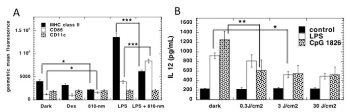
Chen AC, Huang YY, Sharma SK, et al. (2011) Effects of 810-nm laser on murine bone-marrow-derived dendritic cells. Photomed Laser Surg 29: 383–389. doi: 10.1089/pho.2010.2837
![]() |
[45] |
Yamaura M, Yao M, Yaroslavsky I, et al. (2009) Low level light effects on inflammatory cytokine production by rheumatoid arthritis synoviocytes. Lasers Surg Med 41: 282–290. doi: 10.1002/lsm.20766
![]() |
[46] |
Hwang MH, Shin JH, Kim KS, et al. (2015) Low level light therapy modulates inflammatory mediators secreted by human annulus fibrosus cells during intervertebral disc degeneration in vitro. Photochem Photobiol 91: 403–410. doi: 10.1111/php.12415
![]() |
[47] |
Imaoka A, Zhang L, Kuboyama N, et al. (2014) Reduction of IL-20 expression in rheumatoid arthritis by linear polarized infrared light irradiation. Laser Ther 23: 109–114. doi: 10.5978/islsm.14-OR-08
![]() |
[48] |
Lim W, Choi H, Kim J, et al. (2015) Anti-inflammatory effect of 635 nm irradiations on in vitro direct/indirect irradiation model. J Oral Pathol Med 44: 94–102. doi: 10.1111/jop.12204
![]() |
[49] | Choi H, Lim W, Kim I, et al. (2012) Inflammatory cytokines are suppressed by light-emitting diode irradiation of P. gingivalis LPS-treated human gingival fibroblasts: inflammatory cytokine changes by LED irradiation. Lasers Med Sci 27: 459–467. |
[50] |
Sakurai Y, Yamaguchi M, Abiko Y (2000) Inhibitory effect of low-level laser irradiation on LPS-stimulated prostaglandin E2 production and cyclooxygenase-2 in human gingival fibroblasts. Eur J Oral Sci 108: 29–34. doi: 10.1034/j.1600-0722.2000.00783.x
![]() |
[51] |
Nomura K, Yamaguchi M, Abiko Y (2001) Inhibition of interleukin-1beta production and gene expression in human gingival fibroblasts by low-energy laser irradiation. Lasers Med Sci 16: 218–223. doi: 10.1007/PL00011358
![]() |
[52] |
Briken V, Mosser DM (2011) Editorial: switching on arginase in M2 macrophages. J Leukoc Biol 90: 839–841. doi: 10.1189/jlb.0411203
![]() |
[53] |
Whyte CS, Bishop ET, Ruckerl D, et al. (2011) Suppressor of cytokine signaling (SOCS)1 is a key determinant of differential macrophage activation and function. J Leukoc Biol 90: 845–854. doi: 10.1189/jlb.1110644
![]() |
[54] | Xu H, Wang Z, Li J, et al. (2017) The polarization states of microglia in TBI: A new paradigm for pharmacological intervention. Neural Plast 2017: 5405104. |
[55] | Lu J, Xie L, Liu C, et al. (2017) PTEN/PI3k/AKT regulates macrophage polarization in emphysematous mice. Scand J Immunol. |
[56] |
Saha B, Kodys K, Szabo G (2016) Hepatitis C virus-induced monocyte differentiation into polarized M2 macrophages promotes stellate cell activation via TGF-beta. Cell Mol Gastroenterol Hepatol 2: 302–316. doi: 10.1016/j.jcmgh.2015.12.005
![]() |
[57] | Fernandes KP, Souza NH, Mesquita-Ferrari RA, et al. (2015) Photobiomodulation with 660-nm and 780-nm laser on activated J774 macrophage-like cells: Effect on M1 inflammatory markers. J Photochem Photobiol B 153: 344–351. |
[58] |
Silva IH, de Andrade SC, de Faria AB, et al. (2016) Increase in the nitric oxide release without changes in cell viability of macrophages after laser therapy with 660 and 808 nm lasers. Lasers Med Sci 31: 1855–1862. doi: 10.1007/s10103-016-2061-1
![]() |
[59] |
von Leden RE, Cooney SJ, Ferrara TM, et al. (2013) 808 nm wavelength light induces a dose-dependent alteration in microglial polarization and resultant microglial induced neurite growth. Lasers Surg Med 45: 253–263. doi: 10.1002/lsm.22133
![]() |
[60] | Sousa KB, de Santana Araujo L, Pedroso NM, et al. (2017) Photobiomodulation effects on gene and protein expression of proinflammatory chemokines and cytokines by J774 macrophages polarized to M1 phenotype. Lasers Surg Med 49: 36. |
[61] | de Lima FJ, de Oliveira Neto OB, Barbosa FT, et al. (2016) Is there a protocol in experimental skin wounds in rats using low-level diode laser therapy (LLDLT) combining or not red and infrared wavelengths? Systematic review. Lasers Med Sci 31: 779–787. |
[62] | Tchanque-Fossuo CN, Ho D, Dahle SE, et al. (2016) Low-level light therapy for treatment of diabetic foot ulcer: a review of clinical experiences. J Drugs Dermatol 15: 843–848. |
[63] |
Gupta A, Keshri GK, Yadav A, et al. (2015) Superpulsed (Ga-As, 904 nm) low-level laser therapy (LLLT) attenuates inflammatory response and enhances healing of burn wounds. J Biophotonics 8: 489–501. doi: 10.1002/jbio.201400058
![]() |
[64] |
Weylandt KH, Chiu CY, Gomolka B, et al. (2012) Omega-3 fatty acids and their lipid mediators: towards an understanding of resolvin and protectin formation. Prostag Oth Lipid M 97: 73–82. doi: 10.1016/j.prostaglandins.2012.01.005
![]() |
[65] |
Tang Y, Zhang MJ, Hellmann J, et al. (2013) Proresolution therapy for the treatment of delayed healing of diabetic wounds. Diabetes 62: 618–627. doi: 10.2337/db12-0684
![]() |
[66] |
Bohr S, Patel SJ, Sarin D, et al. (2013) Resolvin D2 prevents secondary thrombosis and necrosis in a mouse burn wound model. Wound Repair Regen 21: 35–43. doi: 10.1111/j.1524-475X.2012.00853.x
![]() |
[67] |
Castano AP, Dai T, Yaroslavsky I, et al. (2007) Low-level laser therapy for zymosan-induced arthritis in rats: Importance of illumination time. Lasers Surg Med 39: 543–550. doi: 10.1002/lsm.20516
![]() |
[68] |
Moriyama Y, Moriyama EH, Blackmore K, et al. (2005) In vivo study of the inflammatory modulating effects of low-level laser therapy on iNOS expression using bioluminescence imaging. Photochem Photobiol 81: 1351–1355. doi: 10.1562/2005-02-28-RA-450
![]() |
[69] |
Pallotta RC, Bjordal JM, Frigo L, et al. (2012) Infrared (810-nm) low-level laser therapy on rat experimental knee inflammation. Lasers Med Sci 27: 71–78. doi: 10.1007/s10103-011-0906-1
![]() |
[70] | Ferraresi C, Hamblin MR, Parizotto NA (2012) Low-level laser (light) therapy (LLLT) on muscle tissue: performance, fatigue and repair benefited by the power of light. Photonics Lasers Med 1: 267–286. |
[71] | Ferraresi C, Huang YY, Hamblin MR (2016) Photobiomodulation in human muscle tissue: an advantage in sports performance? J Biophotonics. |
[72] |
Ferraresi C, de Sousa MV, Huang YY, et al. (2015) Time response of increases in ATP and muscle resistance to fatigue after low-level laser (light) therapy (LLLT) in mice. Lasers Med Sci 30: 1259–1267. doi: 10.1007/s10103-015-1723-8
![]() |
[73] |
Silveira PC, Scheffer Dda L, Glaser V, et al. (2016) Low-level laser therapy attenuates the acute inflammatory response induced by muscle traumatic injury. Free Radic Res 50: 503–513. doi: 10.3109/10715762.2016.1147649
![]() |
[74] |
Pires de Sousa MV, Ferraresi C, Kawakubo M, et al. (2016) Transcranial low-level laser therapy (810 nm) temporarily inhibits peripheral nociception: photoneuromodulation of glutamate receptors, prostatic acid phophatase, and adenosine triphosphate. Neurophotonics 3: 015003. doi: 10.1117/1.NPh.3.1.015003
![]() |
[75] |
de Sousa MV, Ferraresi C, de Magalhaes AC, et al. (2014) Building, testing and validating a set of home-made von Frey filaments: A precise, accurate and cost effective alternative for nociception assessment. J Neurosci Methods 232: 1–5. doi: 10.1016/j.jneumeth.2014.04.017
![]() |
[76] | Kobiela Ketz A, Byrnes KR, Grunberg NE, et al. (2016) Characterization of Macrophage/Microglial activation and effect of photobiomodulation in the spared nerve injury model of neuropathic pain. Pain Med: pnw144. |
[77] |
Decosterd I, Woolf CJ (2000) Spared nerve injury: an animal model of persistent peripheral neuropathic pain. Pain 87: 149–158. doi: 10.1016/S0304-3959(00)00276-1
![]() |
[78] |
de Lima FM, Vitoretti L, Coelho F, et al. (2013) Suppressive effect of low-level laser therapy on tracheal hyperresponsiveness and lung inflammation in rat subjected to intestinal ischemia and reperfusion. Lasers Med Sci 28: 551–564. doi: 10.1007/s10103-012-1088-1
![]() |
[79] |
Silva VR, Marcondes P, Silva M, et al. (2014) Low-level laser therapy inhibits bronchoconstriction, Th2 inflammation and airway remodeling in allergic asthma. Respir Physiol Neurobiol 194: 37–48. doi: 10.1016/j.resp.2014.01.008
![]() |
[80] | Rigonato-Oliveira N, Brito A, Vitoretti L, et al. (2017) Effect of low-level laser therapy on chronic lung inflammation in experimental model of asthma: A comparative study of doses. Lasers Surg Med 49: 36. |
[81] |
Huang YY, Gupta A, Vecchio D, et al. (2012) Transcranial low level laser (light) therapy for traumatic brain injury. J Biophotonics 5: 827–837. doi: 10.1002/jbio.201200077
![]() |
[82] |
Thunshelle C, Hamblin MR (2016) Transcranial low-level laser (light) therapy for brain injury. Photomed Laser Surg 34: 587–598. doi: 10.1089/pho.2015.4051
![]() |
[83] |
Hamblin MR (2016) Shining light on the head: Photobiomodulation for brain disorders. BBA Clin 6: 113–124. doi: 10.1016/j.bbacli.2016.09.002
![]() |
[84] |
Khuman J, Zhang J, Park J, et al. (2012) Low-level laser light therapy improves cognitive deficits and inhibits microglial activation after controlled cortical impact in mice. J Neurotrauma 29: 408–417. doi: 10.1089/neu.2010.1745
![]() |
[85] |
Veronez S, Assis L, Del Campo P, et al. (2017) Effects of different fluences of low-level laser therapy in an experimental model of spinal cord injury in rats. Lasers Med Sci 32: 343–349. doi: 10.1007/s10103-016-2120-7
![]() |
[86] |
Muili KA, Gopalakrishnan S, Eells JT, et al. (2013) Photobiomodulation induced by 670 nm light ameliorates MOG35-55 induced EAE in female C57BL/6 mice: a role for remediation of nitrosative stress. PLoS One 8: e67358. doi: 10.1371/journal.pone.0067358
![]() |
[87] |
Yoshimura TM, Sabino CP, Ribeiro MS (2016) Photobiomodulation reduces abdominal adipose tissue inflammatory infiltrate of diet-induced obese and hyperglycemic mice. J Biophotonics 9: 1255–1262. doi: 10.1002/jbio.201600088
![]() |
[88] |
Bjordal JM, Lopes-Martins RA, Iversen VV (2006) A randomised, placebo controlled trial of low level laser therapy for activated Achilles tendinitis with microdialysis measurement of peritendinous prostaglandin E2 concentrations. Br J Sports Med 40: 76–80. doi: 10.1136/bjsm.2005.020842
![]() |
[89] |
Hofling DB, Chavantes MC, Juliano AG, et al. (2010) Low-level laser therapy in chronic autoimmune thyroiditis: a pilot study. Lasers Surg Med 42: 589–596. doi: 10.1002/lsm.20941
![]() |
[90] |
Hofling DB, Chavantes MC, Juliano AG, et al. (2013) Low-level laser in the treatment of patients with hypothyroidism induced by chronic autoimmune thyroiditis: a randomized, placebo-controlled clinical trial. Lasers Med Sci 28: 743–753. doi: 10.1007/s10103-012-1129-9
![]() |
[91] | Hofling DB, Chavantes MC, Juliano AG, et al. (2012) Assessment of the effects of low-level laser therapy on the thyroid vascularization of patients with autoimmune hypothyroidism by color Doppler ultrasound. ISRN Endocrinol 2012: 126720. |
[92] |
Hofling DB, Chavantes MC, Acencio MM, et al. (2014) Effects of low-level laser therapy on the serum TGF-beta1 concentrations in individuals with autoimmune thyroiditis. Photomed Laser Surg 32: 444–449. doi: 10.1089/pho.2014.3716
![]() |
[93] | Hofling D, Chavantes MC, Buchpiguel CA, et al. (2017) Long-term follow-up of patients with hypothyroidism induced by autoimmune thyroiditis submitted to low-level laser therapy. Lasers Surg Med 49: 36. |
[94] | Ferraresi C, Beltrame T, Fabrizzi F, et al. (2015) Muscular pre-conditioning using light-emitting diode therapy (LEDT) for high-intensity exercise: a randomized double-blind placebo-controlled trial with a single elite runner. Physiother Theory Pract: 1–8. |
[95] |
Ferraresi C, Dos Santos RV, Marques G, et al. (2015) Light-emitting diode therapy (LEDT) before matches prevents increase in creatine kinase with a light dose response in volleyball players. Lasers Med Sci 30: 1281–1287. doi: 10.1007/s10103-015-1728-3
![]() |
[96] |
Pinto HD, Vanin AA, Miranda EF, et al. (2016) Photobiomodulation therapy improves performance and accelerates recovery of high-level rugby players in field test: A randomized, crossover, double-blind, placebo-controlled clinical study. J Strength Cond Res 30: 3329–3338. doi: 10.1519/JSC.0000000000001439
![]() |
[97] |
Ferraresi C, Bertucci D, Schiavinato J, et al. (2016) Effects of light-emitting diode therapy on muscle hypertrophy, gene expression, performance, damage, and delayed-onset muscle soreness: case-control study with a pair of identical twins. Am J Phys Med Rehabil 95: 746–757. doi: 10.1097/PHM.0000000000000490
![]() |
[98] | Johnston A, Xing X, Wolterink L, et al. (2016) IL-1 and IL-36 are dominant cytokines in generalized pustular psoriasis. J Allergy Clin Immunol. |
[99] |
Ablon G (2010) Combination 830-nm and 633-nm light-emitting diode phototherapy shows promise in the treatment of recalcitrant psoriasis: preliminary findings. Photomed Laser Surg 28: 141–146. doi: 10.1089/pho.2009.2484
![]() |
[100] |
Choi M, Na SY, Cho S, et al. (2011) Low level light could work on skin inflammatory disease: a case report on refractory acrodermatitis continua. J Korean Med Sci 26: 454–456. doi: 10.3346/jkms.2011.26.3.454
![]() |
[101] |
Hamblin MR (2013) Can osteoarthritis be treated with light? Arthritis Res Ther 15: 120. doi: 10.1186/ar4354
![]() |
[102] |
Ip D (2015) Does addition of low-level laser therapy (LLLT) in conservative care of knee arthritis successfully postpone the need for joint replacement? Lasers Med Sci 30: 2335–2339. doi: 10.1007/s10103-015-1814-6
![]() |
[103] | Brosseau L, Robinson V, Wells G, et al. (2005) Low level laser therapy (Classes I, II and III) for treating rheumatoid arthritis. Cochrane Database Syst Rev 19: CD002049. |
[104] | Brosseau L, Welch V, Wells G, et al. (2004) Low level laser therapy (Classes I, II and III) for treating osteoarthritis. Cochrane Database Syst Rev: CD002046. |
[105] |
Barabas K, Bakos J, Zeitler Z, et al. (2014) Effects of laser treatment on the expression of cytosolic proteins in the synovium of patients with osteoarthritis. Lasers Surg Med 46: 644–649. doi: 10.1002/lsm.22268
![]() |
[106] | Gregoriou S, Papafragkaki D, Kontochristopoulos G, et al. (2010) Cytokines and other mediators in alopecia areata. Mediators Inflamm 2010: 928030. |
[107] |
Avci P, Gupta GK, Clark J, et al. (2014) Low-level laser (light) therapy (LLLT) for treatment of hair loss. Lasers Surg Med 46: 144-151. doi: 10.1002/lsm.22170
![]() |
[108] |
Gupta AK, Foley KA (2017) A critical assessment of the evidence for low-level laser therapy in the treatment of hair loss. Dermatol Surg 43: 188–197. doi: 10.1097/DSS.0000000000000904
![]() |
[109] |
Yamazaki M, Miura Y, Tsuboi R, et al. (2003) Linear polarized infrared irradiation using Super Lizer is an effective treatment for multiple-type alopecia areata. Int J Dermatol 42: 738–740. doi: 10.1046/j.1365-4362.2003.01968.x
![]() |
1. | Nabeela Anwar, Aqsa Ghaffar, Muhammad Asif Zahoor Raja, Iftikhar Ahmad, Muhammad Shoaib, Adiqa Kausar Kiani, Stochastic supervised neuro-architecture design for analyzing vector-borne plant virus epidemics with latency and incubation effects, 2024, 139, 2190-5444, 10.1140/epjp/s13360-024-05883-9 |