Persons enduring serious mental illness (SMI) and living in supported housing facilities often receive inadequate care, which can negatively impact their health outcomes. To address these challenges, it is crucial to prioritize interventions that promote personal recovery and address the unique needs of this group. When developing effective, equitable, and relevant interventions, it is essential to consider the experiences of persons with an SMI. By incorporating their perspectives, we can enhance the understanding, and thereby, the design and implementation of activity- and recovery-oriented interventions that promote health, quality of life, and social connectedness in this vulnerable population. Thus, the aim of this study is to explore the stories of participants partaking in Everyday Life Rehabilitation and how they make sense of their engagements in everyday life activities and their recovery processes.
Applying a narrative analysis, this study explores the stories of seven individuals with an SMI residing in Swedish supported housing facilities, participating in the Everyday Life Rehabilitation (ELR) program during six months, and how they retrospectively make meaning of their engagement in everyday life activities and recovery processes.
The participants' stories about their rehabilitation and personal recovery pathways elucidate how the inherent power of the activity, as well as the support the participants received to get started and succeed, had a significant impact on their self-identity, confidence, motivation, mattering, life prospects, and vitality. The participants valued the transparent steps along the process, weekly meetings, the signals, beliefs, and feedback communicated throughout, and the persistent, adaptive, and yet supporting approach in their personal progress.
This study underscores the need for interventions that prioritize meaningful activities and are sensitive to the complexity of the personal recovery process, especially in supported housing facilities. Future research should further explore effective strategies and mechanisms to promote personal recovery and to reduce the stigma associated with SMI.
Citation: Rosaline Bezerra Aguiar, Maria Lindström. Stories of taking part in Everyday Life Rehabilitation - A narrative inquiry of residents with serious mental illness and their recovery pathway[J]. AIMS Public Health, 2024, 11(4): 1198-1222. doi: 10.3934/publichealth.2024062
Persons enduring serious mental illness (SMI) and living in supported housing facilities often receive inadequate care, which can negatively impact their health outcomes. To address these challenges, it is crucial to prioritize interventions that promote personal recovery and address the unique needs of this group. When developing effective, equitable, and relevant interventions, it is essential to consider the experiences of persons with an SMI. By incorporating their perspectives, we can enhance the understanding, and thereby, the design and implementation of activity- and recovery-oriented interventions that promote health, quality of life, and social connectedness in this vulnerable population. Thus, the aim of this study is to explore the stories of participants partaking in Everyday Life Rehabilitation and how they make sense of their engagements in everyday life activities and their recovery processes.
Applying a narrative analysis, this study explores the stories of seven individuals with an SMI residing in Swedish supported housing facilities, participating in the Everyday Life Rehabilitation (ELR) program during six months, and how they retrospectively make meaning of their engagement in everyday life activities and recovery processes.
The participants' stories about their rehabilitation and personal recovery pathways elucidate how the inherent power of the activity, as well as the support the participants received to get started and succeed, had a significant impact on their self-identity, confidence, motivation, mattering, life prospects, and vitality. The participants valued the transparent steps along the process, weekly meetings, the signals, beliefs, and feedback communicated throughout, and the persistent, adaptive, and yet supporting approach in their personal progress.
This study underscores the need for interventions that prioritize meaningful activities and are sensitive to the complexity of the personal recovery process, especially in supported housing facilities. Future research should further explore effective strategies and mechanisms to promote personal recovery and to reduce the stigma associated with SMI.
Connectedness, Hope, Identity, Meaning, and Empowerment
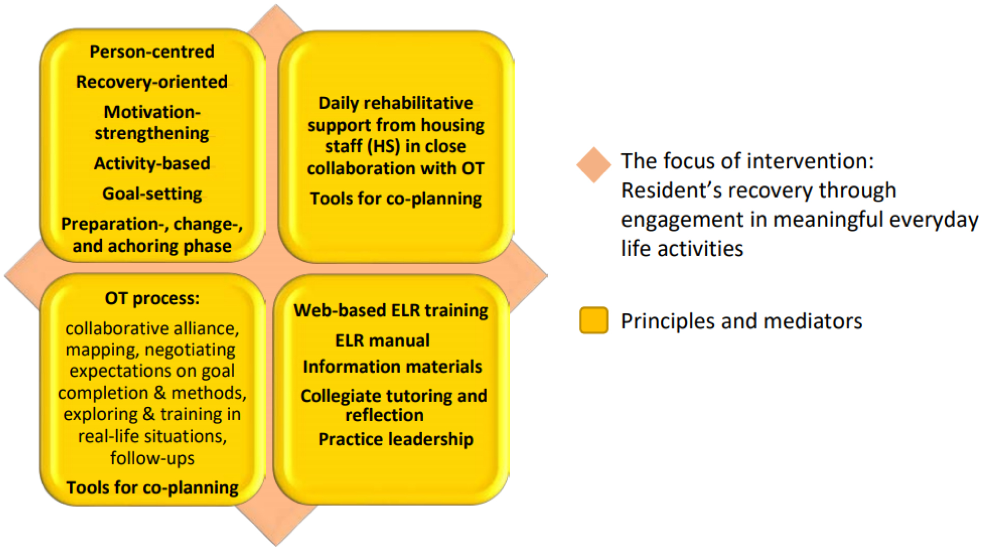
Everyday Life Rehabilitation
Housing staff
Occupational Therapist
Physiotherapist
Randomized Controlled Trial
Sustainable Development Goals
Serious mental illness
Simple Taxonomy for Supported Accommodation
Years lived with disability

| [1] | Centers for Disease Control and Prevetion (CDC)About Mental Health (2022). Available from: https://www.cdc.gov/mentalhealth/ |
| [2] |
Votruba N, Thornicroft G (2016) Sustainable development goals and mental health: learnings from the contribution of the FundaMentalSDG global initiative. Glob Ment Health 3: e26. https://doi.org/10.1017/gmh.2016.20 
|
| [3] | Dybdahl R, Lien L (2017) Mental health is an integral part of the sustainable development goals. Prev Med Comm Health 1: 1-3. https://doi.org/10.15761/PMCH.1000104 |
| [4] | World Health Organization (WHO)World mental health report: transforming mental health for all (2022). Available from: https://www.who.int/publications/i/item/9789240049338 |
| [5] | Bloom DE, Cafiero E, Jané-Llopis E, et al. (2012) The global economic burden of noncommunicable diseases. Program on the Global Demography of Aging. |
| [6] | Global Burden of Disease Collaborative Network (2020) Global Burden of Disease Study 2019 (GBD 2019) Disability Weights. Seattle, United States of America: Institute for Health Metrics and Evaluation (IHME). https://doi.org/10.6069/1W19-VX76 |
| [7] |
Lipskaya-Velikovsky L, Elgerisi D, Easterbrook A, et al. (2019) Motor skills, cognition, and work performance of people with severe mental illness. Disabil Rehab 41: 1396-1402. https://doi.org/10.1080/09638288.2018.1425744
|
| [8] |
Sarsour K, Morin CM, Foley K, et al. (2010) Association of insomnia severity and comorbid medical and psychiatric disorders in a health plan-based sample: insomnia severity and comorbidities. Sleep Med 11: 69-74. https://doi.org/10.1016/j.sleep.2009.02.008
|
| [9] |
Egbe CO, Brooke-Sumner C, Kathree T, et al. (2014) Psychiatric stigma and discrimination in South Africa: perspectives from key stakeholders. BMC Psychiatry 14: 1-14. https://doi.org/10.1186/1471-244X-14-191
|
| [10] |
Nagle S, Cook JV, Polatajko HJ (2002) I'm doing as much as I can: Occupational choices of persons with a severe and persistent mental illness. J Occ Science 9: 72-81. https://doi.org/10.1080/14427591.2002.9686495
|
| [11] |
Corring DJ, Cook JV (2007) Use of qualitative methods to explore the quality-of-life construct from a consumer perspective. Psych Services 58: 240-244. https://doi.org/10.1176/ps.2007.58.2.240
|
| [12] |
Laursen TM, Nordentoft M, Mortensen PB (2014) Excess early mortality in schizophrenia. Ann Rev Clin Psychol 10: 425-448. https://doi.org/10.1146/annurev-clinpsy-032813-153657
|
| [13] |
Wilmot EG, Edwardson CL, Achana FA, et al. (2012) Sedentary time in adults and the association with diabetes, cardiovascular disease and death: systematic review and meta-analysis. Diabet 55: 2895-2905. https://doi.org/10.1007/s00125-012-2677-z
|
| [14] |
Latoo J, Haddad PM, Mistry M, et al. (2021) The COVID-19 pandemic: an opportunity to make mental health a higher public health priority. BJPpsych Open 7: e172. https://doi.org/10.1192/bjo.2021.1002
|
| [15] | World Health Organization (WHO)Mental health: strengthening our response (2022). Available from: https://www.ccih.org/resource_index/world-health-organization-mental-health-strengthening-our-response/ |
| [16] |
Blount A (2003) Integrated primary care: organizing the evidence. Fam Syst Health 21: 121-133. https://doi.org/10.1037/1091-7527.21.2.121
|
| [17] |
Davidson L, Rowe M, Dileo P, et al. (2021) Recovery-oriented systems of care: A perspective on the past, present, and future. Alcohol Res 41: 9. https://doi.org/10.35946/arcr.v41.1.09
|
| [18] |
Steihaug S, Johannessen AK, Ådnanes M, et al. (2016) Challenges in achieving collaboration in clinical practice: the case of Norwegian health care. Int J Integr Care 16: 3. https://doi.org/10.5334/ijic.2217
|
| [19] | Lindström M, Lindberg M, Sjöström S (2011) Responsiveness or resistance: views of housing staff encountering a new rehabilitation model [dissertation]. Umeå: Umeå University. |
| [20] |
Mojtabai R (2021) US health care reform and enduring barriers to mental health care among low-income adults with psychological distress. Psych Services 72: 338-342. https://doi.org/10.1176/appi.ps.202000194
|
| [21] |
Humphreys K, Lembke A (2014) Recovery-oriented policy and care systems in the UK and USA. Drug Alcohol Rev 33: 13-18. https://doi.org/10.1111/dar.12092
|
| [22] |
Desisto M, Harding CM, McCormick RV, et al. (1995) The Maine and Vermont three-decade studies of serious mental illness: II. Longitudinal course comparisons. Brit J Psych 167: 338-342. https://doi.org/10.1192/bjp.167.3.338
|
| [23] | Anthony WA (1993) Recovery from mental illness: the guiding vision of the mental health service system in the 1990s. Psychosoc Rehab J 16: 11-23. https://doi.org/10.1037/h0095655 |
| [24] |
Slade M, Bird V, Clarke E, et al. (2015) Supporting recovery in patients with psychosis through care by community-based adult mental health teams (REFOCUS): a multisite, cluster, randomised, controlled trial. Lancet Psych 2: 503-514. https://doi.org/10.1016/S2215-0366(15)00086-3
|
| [25] |
Bitter N, Roeg D, Van Assen M, et al. (2017) How effective is the comprehensive approach to rehabilitation (CARe) methodology? A cluster randomized controlled trial. BMC Psych 17: 1-11. https://doi.org/10.1186/s12888-017-1565-y
|
| [26] |
Bergmark M, Bejerholm U, Svensson B, et al. (2018) Complex interventions and interorganisational relationships: examining core implementation components of assertive community treatment. Int J Integr Care 18: 11. https://doi.org/10.5334/ijic.3547
|
| [27] |
Hillborg H, Bergmark M, Bejerholm U (2021) Implementation of individual placement and support in a first-episode psychosis unit: a new way of working. Soc Policy Adm 55: 51-64. https://doi.org/10.1111/spol.12611
|
| [28] |
Bejerholm U, Allaskog C, Andersson J, et al. (2022) Implementation of the Recovery Guide in inpatient mental health services in Sweden - A process evaluation study. Health Exp 25: 1405-1417. https://doi.org/10.1111/hex.13480
|
| [29] |
Roe D, Mashiach-Eizenberg M, Lysaker PH (2011) The relation between objective and subjective domains of recovery among persons with schizophrenia-related disorders. Schizophr Res 131: 133-138. https://doi.org/10.1016/j.schres.2011.05.023
|
| [30] |
Phillips P, Sandford T, Johnston C (2013) Working in mental health: practice and policy in a changing environment. Oxford: Routledge. https://doi.org/10.4324/9780203120910
|
| [31] |
Leamy M, Bird V, Le Boutillier C, et al. (2011) Conceptual framework for personal recovery in mental health: systematic review and narrative synthesis. Brit J Psych 199: 445-452. https://doi.org/10.1192/bjp.bp.110.083733
|
| [32] |
Doroud N, Fossey E, Fortune T (2015) Recovery as an occupational journey: A scoping review exploring the links between occupational engagement and recovery for people with enduring mental health issues. Austr Occ Ther J 62: 378-392. https://doi.org/10.1111/1440-1630.12238
|
| [33] |
Lindström M, Sjöström S, Lindberg M (2013) Stories of rediscovering agency: home-based occupational therapy for people with severe psychiatric disability. Qual Health Res 23: 728-740. https://doi.org/10.1177/1049732313482047
|
| [34] |
Sandhu S, Priebe S, Leavey G, et al. (2017) Intentions and experiences of effective practice in mental health specific supported accommodation services: a qualitative interview study. BMC Health Serv Res 17: 1-13. https://doi.org/10.1186/s12913-017-2411-0
|
| [35] | Lindström M, Hariz GM, Bernspång B (2012) Dealing with real-life challenges: Outcome of a home-based occupational therapy intervention for people with severe psychiatric disability. OTJR 32: 5-14. https://doi.org/10.3928/15394492-20110819-01 |
| [36] | Lindström M (2011) Promoting agency among people with severe psychiatric disability: occupation-oriented interventions in home and community settings [dissertation]. Umeå: Umeå University. |
| [37] |
Eklund M, Argentzell E, Bejerholm U, et al. (2017) Wellbeing, activity and housing satisfaction–comparing residents with psychiatric disabilities in supported housing and ordinary housing with support. BMC Psych 17: 1-12. https://doi.org/10.1186/s12888-017-1472-2
|
| [38] |
Wormdahl I, Husum TL, Rugkåsa J, et al. (2020) Professionals' perspectives on factors within primary mental health services that can affect pathways to involuntary psychiatric admissions. Int J Mental Health Syst 14: 1-12. https://doi.org/10.1186/s13033-020-00417-z
|
| [39] | SocialstyrelsenKompetens i LSS-boenden. [Competence in LSS-housing] (2021). Available from: https://www.socialstyrelsen.se/globalassets/sharepoint-dokument/artikelkatalog/ovrigt/2021-3-7312.pdf |
| [40] |
Malfitano APS, De Souza RGDM, Townsend EA, et al. (2019) Do occupational justice concepts inform occupational therapists' practice? A scoping review. Can J Occ Ther 86: 299-312. https://doi.org/10.1177/0008417419833409
|
| [41] |
Whiteford G, Jones K, Weekes G, et al. (2020) Combatting occupational deprivation and advancing occupational justice in institutional settings: Using a practice-based enquiry approach for service transformation. Brit J Occ Ther 83: 52-61. https://doi.org/10.1177/0308022619865223
|
| [42] | Wilcock AA (2006) An occupational perspective of health. Slack Incorporated . Available from: https://archive.org/details/occupationalpers0000wilc_r6b9/page/n3/mode/2up |
| [43] | Occupational Therapy Australia.OT Australia position statement: occupational deprivation. Austr Occ Ther J (2016) 63: 445-447. https://doi.org/10.1111/1440-1630.12347 |
| [44] | SocialdepartementetThe Swedish Act of Healthcare (2017). Available from: https://rkrattsbaser.gov.se/sfst?bet=2017:30 |
| [45] |
Lindström M, Lindholm L, Liv P (2022) Study protocol for a pragmatic cluster RCT on the effect and cost-effectiveness of Everyday Life Rehabilitation versus treatment as usual for persons with severe psychiatric disability living in sheltered or supported housing facilities. Trials 23: 657. https://doi.org/10.1186/s13063-022-06622-0
|
| [46] | Lindström M (2007) Everyday Life Rehabilitation: manual for integrated activity and recovery-oriented rehabilitation in social psychiatry settings. Umeå: Umeå University. |
| [47] | Lindström M Everyday Life Rehabilitation (ELR): manual 2.0 (Distributed by web-site for the intervention model ELR) (2020). Available from: https://www.everydayliferehabilitation.com/ |
| [48] |
Lindström M (2022) Development of the Everyday Life Rehabilitation model for persons with long-term and complex mental health needs: Preliminary process findings on usefulness and implementation aspects in sheltered and supported housing facilities. Front Psych 13: 954068. https://doi.org/10.3389/fpsyt.2022.954068
|
| [49] |
Ulfseth LA, Josephsson S, Alsaker S (2015) Meaning-making in everyday occupation at a psychiatric centre: A narrative approach. J Occ Science 22: 422-433. https://doi.org/10.1080/14427591.2014.954662
|
| [50] |
Reed NP, Josephsson S, Alsaker S (2020) A narrative study of mental health recovery: exploring unique, open-ended and collective processes. Int J Qual Stud Health Well-being 15: 1747252. https://doi.org/10.1080/17482631.2020.1747252
|
| [51] | Ricoeur P (1991) Life in quest of narrative. London: Routledge. |
| [52] |
Polkinghorne DE (1995) Narrative configuration in qualitative analysis. Int J Qual Stud Edu 8: 5-23. https://doi.org/10.1080/0951839950080103
|
| [53] |
Nhunzvi C, Langhaug L, Mavindidze E, et al. (2020) Occupational justice and social inclusion among people living with HIV and people with mental illness: A scoping review. BMJ Open 10: e036916. https://doi.org/10.1136/bmjopen-2020-036916
|
| [54] | Ricoeur P Time and Narrative (1984). https://doi.org/10.7208/chicago/9780226713519.001.0001 |
| [55] | SocialdepartementetThe Swedish Social Services Act (2001). Available from: https://rkrattsbaser.gov.se/sfst?bet=2001:453 |
| [56] | SocialdepartementetThe Swedish Act concerning Support and Service for Persons with Certain Functional Impairments (1993). Available from: https://rkrattsbaser.gov.se/sfst?bet=1993:387 |
| [57] |
Lilliehorn S, Fjellfeldt M, Högström E, et al. (2023) Contemporary Accommodation Services for People with Psychiatric Disabilities–the Simple Taxonomy for Supported Accommodation (STAX-SA) Applied and Discussed in a Swedish Context. Scand J Disab Res 25: 92-105. https://doi.org/10.16993/sjdr.879
|
| [58] |
McPherson P, Krotofil J, Killaspy H (2018) What works? Toward a new classification system for mental health supported accommodation services: the simple taxonomy for supported accommodation (STAX-SA). IntJ Env Res Public Health 15: 190. https://doi.org/10.3390/ijerph15020190
|
| [59] |
Gallagher M, Muldoon OT, Pettigrew J (2015) An integrative review of social and occupational factors influencing health and wellbeing. Front Psychol 6: 1-11. https://doi.org/10.3389/fpsyg.2015.01281
|
| [60] | Borg M, Karlsson B, Tondora J, et al. (2009) Implementing person-centered care in psychiatric rehabilitation: what does this involve?. Isr J Psychiatry Relat Sci 46: 84-93. |
| [61] |
Lindström M, Isaksson G (2017) Personalized Occupational Transformations: Narratives from Two Occupational Therapists' Experiences with Complex Therapeutic Processes. Occ Ther Ment Health 33: 15-30. https://doi.org/10.1080/0164212X.2016.1194243
|
| [62] | Tondora J, Miller R, Slade M, et al. (2014) Partnering for recovery in mental health: A practical guide to person-centered planning. John Wiley & Sons. |
| [63] |
Hitch D, Pepin G (2021) Doing, being, becoming and belonging at the heart of occupational therapy: An analysis of theoretical ways of knowing. Scand J Occup Ther 28: 13-25. https://doi.org/10.1080/11038128.2020.1726454
|
| [64] |
Sutton DJ, Hocking CS, Smythe LA (2012) A phenomenological study of occupational engagement in recovery from mental illness. Can J Occ Ther 79: 142-150. https://doi.org/10.2182/cjot.2012.79.3.3
|
| [65] |
Killaspy H, Harvey C, Brasier C, et al. (2022) Community-based social interventions for people with severe mental illness: a systematic review and narrative synthesis of recent evidence. World Psych 21: 96-123. https://doi.org/10.1002/wps.20940
|
| [66] |
Hermanski A, Mcclelland J, Pearce-Walker J, et al. (2022) The effects of blue spaces on mental health and associated biomarkers. Int J Ment Health 51: 203-217. https://doi.org/10.1080/00207411.2021.1910173
|
| [67] |
Van Den Berg M, Van Poppel M, Van Kamp I, et al. (2016) Visiting green space is associated with mental health and vitality: A cross-sectional study in four european cities. Health Place 38: 8-15. https://doi.org/10.1016/j.healthplace.2016.01.003
|
| [68] |
Piat M, Seida K, Padgett D (2019) Choice and personal recovery for people with serious mental illness living in supported housing. J Ment Health 29: 306-313. https://doi.org/10.1080/09638237.2019.1581338
|
| [69] |
Greenwood RM, Manning RM (2017) Mastery matters: Consumer choice, psychiatric symptoms and problematic substance use among adults with histories of homelessness. Health Soc Care Community 25: 1050-1060. https://doi.org/10.1111/hsc.12405
|
| [70] |
Slade M, Amering M, Farkas M, et al. (2014) Uses and abuses of recovery: implementing recovery-oriented practices in mental health systems. World Psych 13: 12-20. https://doi.org/10.1002/wps.20084
|
| [71] |
Clarke SP, Crowe TP, Oades LG, et al. (2009) Do goal-setting interventions improve the quality of goals in mental health services?. Psych Rehab J 32: 292-299. https://doi.org/10.2975/32.4.2009.292.299
|
| [72] |
Mishler EG (1986) Research interviewing: Context and narrative. Cambridge, UK: Harvard University Press. https://doi.org/10.4159/9780674041141
|
Figures(1) / Tables(1)

Rosaline Bezerra Aguiar, Maria Lindström. Stories of taking part in Everyday Life Rehabilitation - A narrative inquiry of residents with serious mental illness and their recovery pathway[J]. AIMS Public Health, 2024, 11(4): 1198-1222. doi: 10.3934/publichealth.2024062


 DownLoad: