Figure 1.
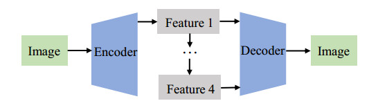
Diagram of the proposed research.


Silicosis is an occupational respiratory disease linked to silica dust inhalation. The main driver was traditional coal mining, but in recent decades, new sources of exposure have emerged. Our aim in this study was to assess the temporal and spatial distribution of mortality due to this disease over a 22-year period in Spain.
Silicosis records, as an Underlying Cause of Death, were extracted from the National Institute of Statistics from 1999 to 2020 using the International Classification of Diseases 10th revision (code J62.8). Age- and sex-adjusted mortality rates per 1,000,000 inhabitants were calculated for the territory and by province. A geographic analysis was performed, and clusters of deaths were identified at the municipal level, and then the outcomes were compared in two periods of 11 years.
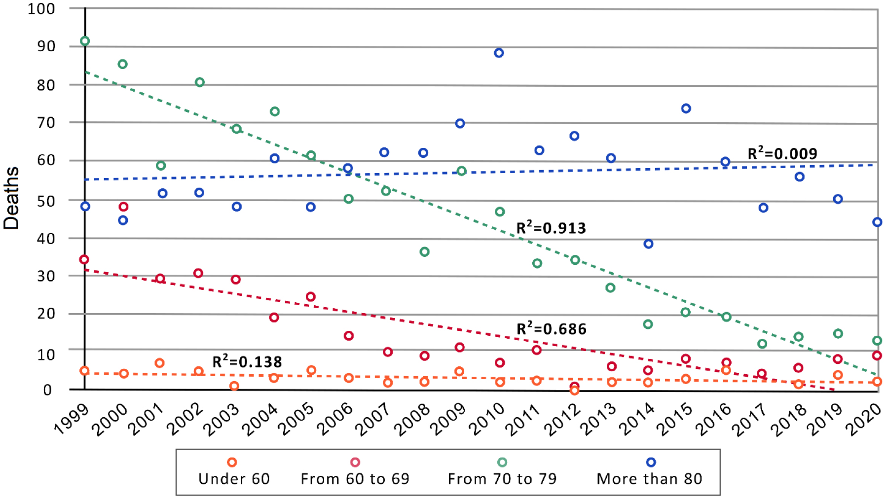
There were 2618 deaths due to silicosis in Spain. The mean age of death increased significantly by 0.66% annually from 1999 to 2013. The age-adjusted mortality rate decreased by 7.30% per year, falling from 3.00 to 0.65 per 1,000,000 inhabitants. The temporal pattern showed a significant decrease of mortality rate in 31% of the provinces (16 out of 52), while it increased in Pontevedra. Regarding the spatial analysis, 11 clusters were found in both periods, but some variations were observed in terms of their distribution in the Spanish territory, as well as in the affected municipalities.
The decrease in mortality due to Silicosis could be related to less exposure to silica dust over the years and an improvement in the survival of those affected. It is thus essential to analyze the role of preventive measures for this occupational disease.
Citation: Germán Sánchez-Díaz, Greta Arias-Merino, Elisa Gallego, Rodrigo Sarmiento-Suárez, Verónica Alonso-Ferreira. Silicosis mortality in Spain (1999–2020): A temporal and geographical approach[J]. AIMS Public Health, 2024, 11(3): 715-728. doi: 10.3934/publichealth.2024036
| [1] | Jingjing Hai, Xian Ling . Normalizer property of finite groups with almost simple subgroups. Electronic Research Archive, 2022, 30(11): 4232-4237. doi: 10.3934/era.2022215 |
| [2] | Jidong Guo, Liang Zhang, Jinke Hai . The normalizer problem for finite groups having normal 2-complements. Electronic Research Archive, 2024, 32(8): 4905-4912. doi: 10.3934/era.2024225 |
| [3] | Xiaoyan Xu, Xiaohua Xu, Jin Chen, Shixun Lin . On forbidden subgraphs of main supergraphs of groups. Electronic Research Archive, 2024, 32(8): 4845-4857. doi: 10.3934/era.2024222 |
| [4] | Huani Li, Xuanlong Ma . Finite groups whose coprime graphs are AT-free. Electronic Research Archive, 2024, 32(11): 6443-6449. doi: 10.3934/era.2024300 |
| [5] | Qiuning Du, Fang Li . Some elementary properties of Laurent phenomenon algebras. Electronic Research Archive, 2022, 30(8): 3019-3041. doi: 10.3934/era.2022153 |
| [6] | Guowei Liu, Hao Xu, Caidi Zhao . Upper semi-continuity of pullback attractors for bipolar fluids with delay. Electronic Research Archive, 2023, 31(10): 5996-6011. doi: 10.3934/era.2023305 |
| [7] | Xue Yu . Orientable vertex imprimitive complete maps. Electronic Research Archive, 2024, 32(4): 2466-2477. doi: 10.3934/era.2024113 |
| [8] | Francisco Javier García-Pacheco, María de los Ángeles Moreno-Frías, Marina Murillo-Arcila . On absolutely invertibles. Electronic Research Archive, 2024, 32(12): 6578-6592. doi: 10.3934/era.2024307 |
| [9] | Sang-Eon Han . Digitally topological groups. Electronic Research Archive, 2022, 30(6): 2356-2384. doi: 10.3934/era.2022120 |
| [10] | Kiyoshi Igusa, Gordana Todorov . Picture groups and maximal green sequences. Electronic Research Archive, 2021, 29(5): 3031-3068. doi: 10.3934/era.2021025 |
Silicosis is an occupational respiratory disease linked to silica dust inhalation. The main driver was traditional coal mining, but in recent decades, new sources of exposure have emerged. Our aim in this study was to assess the temporal and spatial distribution of mortality due to this disease over a 22-year period in Spain.
Silicosis records, as an Underlying Cause of Death, were extracted from the National Institute of Statistics from 1999 to 2020 using the International Classification of Diseases 10th revision (code J62.8). Age- and sex-adjusted mortality rates per 1,000,000 inhabitants were calculated for the territory and by province. A geographic analysis was performed, and clusters of deaths were identified at the municipal level, and then the outcomes were compared in two periods of 11 years.
There were 2618 deaths due to silicosis in Spain. The mean age of death increased significantly by 0.66% annually from 1999 to 2013. The age-adjusted mortality rate decreased by 7.30% per year, falling from 3.00 to 0.65 per 1,000,000 inhabitants. The temporal pattern showed a significant decrease of mortality rate in 31% of the provinces (16 out of 52), while it increased in Pontevedra. Regarding the spatial analysis, 11 clusters were found in both periods, but some variations were observed in terms of their distribution in the Spanish territory, as well as in the affected municipalities.
The decrease in mortality due to Silicosis could be related to less exposure to silica dust over the years and an improvement in the survival of those affected. It is thus essential to analyze the role of preventive measures for this occupational disease.
The COVID-19 outbreak, which began in 2019, is a viral disease caused by severe acute respiratory syndrome coronavirus type 2 (SARS-COV-2) [1,2,3,4]. Most COVID-19 patients have pneumonia, and computed tomography (CT) scans are often used to help doctors diagnose pneumonia in the early stages of COVID-19 outbreaks [5,6,7]. Compared with CT, chest X-ray (CXR) is more widely used in clinical practice because it is easier, faster, and less expensive to perform. However, the sheer volume of CXR data and limited number of physicians cannot ensure that the system operates with maximum efficiency to save more patients [8,9,10,11,12]. A computer-aided system can play a certain auxiliary role [13,14], but its efficiency and accuracy cannot meet the requirements. Improving the accuracy of CXR image lesion identification is still a key issue that urgently needs to be solved.
Traditional methods usually use the mathematical calculation of regions and feature extraction to recognize and classify CXR images. Jaeger et al. [15] proposed an automated method for tuberculosis detection on posterior-anterior chest radiographs. Lung segmentation was modeled as an optimization problem, integrating lung boundaries, regions, shapes, and other attributes with tight segmentation contours and leakage in some areas. Hogeweg et al. [16] combined a texture anomaly detection system running at the pixel level with the clavicle detection system to suppress false-positive reactions, and the pathological structure changed after segmentation, which was detrimental to the judgment of pathology. Candemir et al. [17] proposed a robust lung segmentation method driven by nonrigid registration using a patient-specific adaptive lung model based on image retrieval to detect lung boundaries, achieving an average accuracy of 95.4% on the public JSRT database. However, opacity caused by fluid in the lung space prevents correct detection of lung boundaries. Although regional segmentation has been valued, there is a lack of corresponding supervision mechanisms. To train classifiers that can effectively monitor, Livieris et al. [18] proposed an SSL algorithm for tuberculosis CXR classification, which combines the individual predictions of three commonly used SSL algorithms applying the CST-voting integration principle and voting method. Statistical accuracy was relatively objective, but the process was too tedious. Faced with the problems of complex mathematical principles and low model robustness existing in traditional methods, more cost-effective methods are required in the CXR recognition field.
In recent years, deep learning models such as convolutional neural networks (CNN) [19,20,21,22,23,24,25,26] have been rapidly developed, and they have become the preferred technical means in the field of computer vision. Experts in the medical imaging field have also noted the rapid growth and impact of CNNs. For example, Irfan et al. [27] developed a hybrid deep neural network (HDNN) that uses computed tomography (CT) and X-ray imaging to predict risks. The classification accuracy reached a very high level by training with a dataset on the web along with a regular dataset. The CoVIRNet method proposed by Almalki et al. [28] can automatically diagnose COVID-19 patient images using chest radiographs and alleviate the overfitting problem owing to the small size of the COVID-19 dataset. Most CXR disease recognition methods based on deep-learning technology can be divided into two types. The first type uses a CNN for image segmentation and classification. Shen et al. [26] extracted the symptom part of an image as a block and inputted several different CNNs, and the features obtained were spliced into vectors as the final result. Discriminant features were extracted from alternately stacked layers to capture the heterogeneity of pulmonary nodules; however, the location of the disease could not be directly represented. Rajpurkar et al. [29] developed a 121-layer CNN named CheXNet, which was tested on the ChestX-Ray14 large pneumonia data set containing 14 diseases and achieved an accuracy of more than 0.7 in the classification of diseases. However, the network stacking method is excessively simple, and the image texture is not used more thoroughly. The second type of methods denoise the data to enhance the recognition effect of the other algorithms. Ucar and Korkmaz [30] proposed an architecture based on SqueezeNet to fine-tune COVID-19 diagnosis through raw data enhancement, Bayes optimization, and validation to achieve high accuracy in categorizing COVID-19, pneumonia, and normality. Jiang et al. [31] proposed a residual CNN for denoising COVID-19 images. The residual connection and attention mechanism were used to make the network pay more attention to the texture details of the CXR images, and the effect of the denoised images was significantly improved in the COVID-19 recognition task.
Waheed et al. [32] used an adversarial network model to synthesize CXR images, which allowed the model to rely on external information to improve the sample quality, thus increasing the number of images of COVID-19 symptoms. However, the recognition task was limited to classification, and the location of the symptoms was not accurately obtained. In a more specialized work, Jaiswal et al. [33] applied the target detection algorithm to the RSNA pneumonia data set, and obtained an optimal accuracy by fusing the prediction boundary boxes of multiple models. Because of its large memory occupation and use of a single category of dataset, the detection results of diversified diseases cannot be determined. This provides the motivation and references for our work.
Although the accuracy of the above methods continues to improve, there are still some obvious shortcomings: 1) most of them are classification and segmentation methods, and lack intuitive target boxes to directly indicate the location of symptoms, so the evaluation efficiency needs to be improved. 2) The ideal accuracy usually requires the fusion of the detection effects of multiple models, which occupies a large memory and is not realistic in practical applications. 3) The CXR data volume of COVID-19 is small, and it is a single category, so generalization results cannot be obtained. To solve the above problems, a lesion detection method based on a scalable attention residual CNN is proposed in this paper. A variety of convolution kernel sizes are used to obtain a variety of resolutions, and adaptive global attention is used to extract the spatial features of each resolution and connect them. A feature fusion method with different tree-structure depths is designed. Finally, the attention mechanism is used to fuse the spatial and channel information. All the effects were tested in a single model using the VinDr-CXR dataset. The main contributions of this study are summarized as follows:
● To improve the ability of the deep learning model in CXR target detection, we propose a CNN model and construct a structure based on the model that can effectively improve the accuracy of CXR location detection and improve the sensitivity of the model to CXR features from the aspects of attention and feature fusion.
● We use zero-based training to customize our CNN model for the data set, and the training effect of a single model can outperform most of the classical deep learning models. The development of CXR data sets containing target location information became the focus, proving the necessity and advance of our work and providing the corresponding references for future work.
● The three modules designed in this study, multi-convolution feature fusion block (MFFB), tree-structured aggregation module (TSAM), and scalable channel and spatial attention (SCSA), can effectively improve the detection effect of the deep learning model in CXR, and the accuracy increases from 12.83 to 15.75% after the addition of the modules, higher than that obtained by the existing mainstream target detection model.
We summarized our research into three parts: encoder, multiple feature blocks, and decoder, simplifying the complex model structure. The encoder in Figure 1 represents the scalable attention residual CNN (SAR-CNN), whereas the decoder is a simple convolutional layer. As many as four feature blocks, from Features 1–4, are input into the decoder in the form of pyramids, and finally, the positioning of the detection frame and judgment of the lesion category are performed. In the following sections, we introduce the proposed CXR target detection network, SAR-CNN, in detail, including the MFFB, TSAM and SCSA modules. These modules are independent and embeddable and can be migrated to common convolutional networks. The MFFB is designed to interpret CXR image information from a multi-resolution perspective, whereas the TSAM utilizes the characteristics of the tree structure to perform left-right branch and multi-level feature fusion, and finally the SCSA is used for spatial and channel attention integration. Residual modules [34] are used in the rest of the network to improve its learnability. Details of the SAR-CNN training are covered in the next section.
The proposed SAR-CNN network structure composed of MFFB, TSAM and SCSA is shown in Figure 2. The VGG [35] straight-cylinder module stacking method was adopted to improve the embeddability of modules. The predictive image (input) was input to the CNN in 512 × 512 size. Four feature graphs are output and sent for feature post-processing through the modules mentioned in the following sections. It can be observed from the CAM graph that the four feature maps have different degrees of performance in characterization feature fitting. The neck and head parts in RefineDet [36] have both first-stage and second-stage advantages, so we replace the backbone network of RefineDet with SAR-CNN and finally obtain the final detection result (output) of our predicted image. Such a framework will not only help improve the localization performance, but also, by means of attention, provide a way to explain visually the model decisions, both of which are important for the clinical deployment of deep learning models.

As shown in Figure 3, we propose an MFBB that is different from the simple connection and fusion of existing algorithms. M1, M2 and M3 were obtained by 3 × 3, 5 × 5 and 7 × 7 convolution kernel extractions of Min∈RC×H×W, where M1∈RC×H×W was extracted using the same mode convolution. We used ECA-Net [37], which is a simple and effective attention processing method. The difference is that we used the convolution of more receptive fields to extract richer feature scales and used global average pooling (GAP) to extract features along channel dimensions from M2 and M3 with different resolutions. Next, 1D convolution was used for adaptive feature extraction. After the sigmoid, channel attention S2∈R1×1×C and S3∈R1×1×C were obtained, and the fusion function F(.) defined in Formula (2.1) is adopted. The final output feature of the module Mout∈RC×H×W was obtained.
| Mout=F(M1⊗S2⊗S3)=σ( BatchNorm ( Conv 3×3(M1⊗S2⊗S3))), | (2.1) |

where F(.) represents a combination of three layers: the same mode 3 × 3 convolution layer, the BatchNorm layer [38], and the nonlinear activation function ReLU [39]. ⊗ is the element-wise multiplication, σ represents the ReLU layer, and Conv3×3 is the same-mode convolution layer of 3 × 3 size. The convolution layer is used to fuse feature graphs and channel attention of two different resolutions to avoid the feature mismatch of related images caused by simple multiplication. BatchNorm is a normalization method that solves the phenomenon of inconsistent distribution of input data, highlights the relative difference in distribution between them, and speeds up training. The ReLU layer adds a nonlinear relationship to the feature layer to avoid gradient disappearance and over-fitting, which ensures that our neural network can complete complex tasks.
We designed the TSAM by summarizing the feature fusion methods of DenseNet [40] and FPN [41] and drawing inspiration from the DLA structure [42], as shown in Figure 4.

In contrast to DLA, we adopt a fixed number of layers and use feature layers with more details to avoid the overfitting problems caused by excessively deep iterative networks. Each structural unit corresponds to a residual module. For simplicity and resource saving, this residual module contains only two 3 × 3 convolution and BatchNorm layers. Each aggregation node adopts a 3 × 3 convolution, BatchNorm layer, and ReLU, and the features of the left and right branches are fused to obtain the feature graph:
| A(x1,x2)=σ(BatchNorm(W1x1+W2x2+b))=σ(BatchNorm(W1x1+W2(W0x1+b0)+b)), | (2.2) |
where x1 and x2 represent the left- and right-branch features of the binary tree before fusion, respectively. σ represents a nonlinear ReLU. W and b respectively represent the weights and offsets of convolution, and x2 is obtained by x1 through a structural unit. The TSAM combines layers of different depths to learn richer combinations that span more feature layers.
This module utilizes both the channel and spatial dimensions of attention, and we use SCSA as a transitional stage between the two modules, as shown in Figure 5. In the channel dimension module, Minput is input into two paths to obtain MS∈R1×H×W and MC∈RC×1×1, respectively, and MSCSA∈RC×H×W is obtained by combining them. Then, residual fusion is performed between Minput∈RC×H×W MSCSA, respectively.
| Moutput =Minput +Minput ⊗MSCSA =Minput +Minput ⊗σ(MS+MC), | (2.3) |

where σ is the sigmoid function and ⊗ is element-wise multiplication. In the channel attention module, the channel information encoded in two different ways is obtained through global average pooling and global maximum pooling. In addition, a full-connection layer is set as Share FC to interact with the information of the two channels, and the feature size obtained is RC/r×1×1. After the BatchNorm layer, the two are added.
| Mc=BN( ShareFC ( GAP (Minput )))+BN( ShareFC ( GMP (Minput ))), | (2.4) |
where BN is the batch normalization layer. The spatial-dimension module compresses Minput∈RC×H×W to RC/r×H×W through a layer of 1 × 1 convolution. A layer of 3 × 3 dilated convolution is set to expand the receptive field to utilize more contextual information, and then a layer of the spatial attention map MS∈R1×H×W is obtained through a layer of 1 × 1 convolution. Finally, a batch normalization layer is used to adjust the search space:
| MS=BN(Conv1×1(Conv3×3(Conv1×1(Minput )))), | (2.5) |
where BN is the batch normalization layer, Conv is the convolution layer, and the superscript is the size of the convolution kernel. In addition, the SCSA module is followed by MaxPooling of a layer with a size of 2 × 2 and a stride of 2 as the lower sampling layer. SCSA has a working principle similar to that of BAM [43], but it uses the different global pooling features of GAP and GMP to extract channel attention and has more types of channel feature maps. Compared to CBAM [44], the original features were added after the fusion of the channel and spatial attention, rather than in sequence. SCSA prefers to combine the advantages of BAM and CBAM, and discard unnecessary parts.
We observed that the residual structure plays a key role in medical image detection tasks. Therefore, in addition to the three modules proposed in this study, residual modules were used in the rest of the network to sort out the features obtained by fitting the above three modules and further improve the robustness of the network. The residual module is derived from ResNet, which adds jump connections to the convolutional module to solve the problems of gradient disappearance and gradient explosion during the training of deep neural networks, as shown in Figure 6. In addition, we observed that the residual module could correlate features of different scales. In special cases, the disease regions in CXR will cross and even overlap, and the use of a residual module can help correlate features of overlapping target regions.

As the COVID-19 dataset is not publicly available on a large scale, it is too small and of poor quality, even if it is partially curated and annotated. For the above reasons, we selected the common CXR dataset that meets the requirements, that is, the VinDr-CXR dataset. VinDr-CXR is a chest radiography dataset published by the Vingroup Big Data Institute (VinBigdata) [45] and is currently the largest public CXR dataset with radiologist-generated annotations in both the training and test sets. Collected from the Hospital 108 (H108) and the Hanoi Medical University Hospital (HMUH), 18000 CXR data were manually annotated by 17 professional radiologists. Furthermore, the VinDr-CXR dataset was divided into a 15,000 image training set and a 3000 image test set. The training set was independently annotated by three doctors and the test set was jointly annotated by five doctors. Because of the low number of images in eight of the 22 categories containing local location information, we incorporated these eight minor categories into the other lesions, and thus our task was defined as the target detection problem of 14 lesions. The names and quantity statistics of the different categories in the VinDr-CXR dataset are shown in Figure 7.

The proposed method was trained and tested on the Pytorch framework [46], and the relative hyperparameters of the network were based on ScratchDet [47], with a learning rate of 0.05, using SGD with 0.0005 weight decay and 0.9 momentum. The batch size was set to eight, and the training wheel number adaptive adjustment mechanism was adopted. The experiment was interrupted when the accuracy of more than 150 epochs did not exceed the highest accuracy for five consecutive epochs. The number of decreased rounds was 50, 100 and 150, respectively, and the reduction at each time was 1/10. The resolution of the image input was 512 × 512, and the SSD was used for data enhancement (random expansion, clipping, inversion, random photometric distortion, etc.). All the convolution layers were initialized using the Xavier uniform method. The comparative experimental algorithms were tested using pre-training weights in the Pytorch framework, and the number of training rounds was uniformly set to 300. The first 20 rounds frozen the trunk network. In addition, each round was verified and the weight was saved. Every 50 rounds, a weight was selected for the accuracy test, and the highest accuracy was used as the comparative experimental data.
Network training involves loss functions and optimizers using RefineDet parameter requirements. To imitate the prediction process of the two-stage target detection algorithm, the loss function LSAR consists of LA and LB, where LA corresponds to the stage of the position and size of the target in the returned image and LB determines the category of the target according to the returned target. NARM and NODM in the formula are the numbers of positive anchors in ARM and ODM, respectively. In particular, i is the index of each anchor box and the smooth L1 loss is used as LS, and si is used to judge whether the predicted category is consistent with the ground truth label; the match is 1; otherwise, it is 0, and the ground truth is represented by g*i.
In Formula (3.1), pi and xi are the probability and corresponding position coordinates of the target in ARM anchor boxes i, respectively, and Lb uses the cross-entropy loss over two classes as a dichotomous loss function.
| LA=1NARM(∑Lb(pi,Si)+∑siLs(xi,g∗)). | (3.1) |
In Formula (3.2), ci and ti are the categories of the ODM anchor boxes i and the corresponding coordinates of the bounding box, respectively, whereas li is the ground truth class label of the anchor. Lm uses the softmax loss over multiple class confidences as a multiclass classification loss.
| LB=1NODM(∑Lm(ci,li)+∑SiLs(ti,g∗i)). | (3.2) |
The final value of the entire loss function can be obtained by adding the values of the two aforementioned loss functions.
| LSAR=LA+LB. | (3.3) |
To prove the validity of the trunk network we designed, we performed several comparative experiments on the trunk network: 1) VGG-16 in RefineDet source code; 2) on the basis of 1), a BN layer was added to each convolutional layer as a combination; and 3) the original VGG-16 was replaced with other common backbone networks. The experimental results are listed in Table 1. The precision of the trunk network designed by us was higher than that of other experiments. Although the number of parameters was reduced after the replacement of some trunk networks, the corresponding precision was too low and did not have the functional effect required by the task. After the analysis, we believe that although VGG, ResNet, DLA, and other trunk networks are frequently used as a means to improve the task effect, they are essentially designed for classification, which is different from our CXR target detection task, resulting in poor performance. The trunk network we designed increased the number of parameters within the allowed range, thus obtaining a 15.75% mAP, which is higher than the accuracy of the other versions, proving the effectiveness of our network in handling this task.
| Backbone | mAP@0.5(%) | Inference speed (fps) | Params (M) |
| VGG-16 | 12.83 | 9.96 | 34.27 |
| VGG-16+BN | 13.67 | 8.50 | 34.28 |
| ResNet-18 | 8.05 | 4.62 | 22.75 |
| ResNet-34 | 8.25 | 3.32 | 32.85 |
| DLA-60 | 8.54 | 7.98 | 33.90 |
| DLA-102 | 9.00 | 5.86 | 45.30 |
| SAR-CNN (Ours) | 15.75 | 2.60 | 56.48 |
 DownLoad:
CSV
DownLoad:
CSV
According to the modules proposed in Section 2, we conducted the corresponding combined experiments to show the contribution and role of each module to the whole. A tick indicates that the network applies to the module. The experimental results are listed in Table 2. For single-module embedding, two-module combination, or three-module embedding, the accuracy can be further improved. To fit the information of the finishing module, ResBlock was added, and the accuracy of the network was finally improved to 15.75%. We believe that the three specially designed modules improve the robustness of the overall network for the following reasons: First, features of multiple resolutions are conducive to the formation of relatively rich image information, especially for sites with subtle lesions. Second, a simple and effective topological structure is needed to fuse medical image features with insufficient information. Third, medical images require the network to apply attention mechanisms from different angles.
| Component | SAR-CNN | ||||||||
| MFFB | ✓ | ✓ | ✓ | ✓ | ✓ | ||||
| TSAM | ✓ | ✓ | ✓ | ✓ | ✓ | ||||
| SCSA | ✓ | ✓ | ✓ | ✓ | ✓ | ||||
| ResBlock | ✓ | ||||||||
| mAP@0.5(%) | 15.75 | 14.20 | 13.18 | 13.49 | 13.15 | 13.11 | 13.12 | 13.08 | 12.83 |
DownLoad:
CSV
To prove the superiority of our method, we used the PASCAL VOC 2010 standard [48] and IoU > 0.4 (0.5, 0.6, 0.7 and 0.8), and compared the mAP index with the mainstream target detection model. The experimental results are presented in Table 3. In CenterNet, owing to the special setting of non-maximum suppression (NMS), the value of IoU does not affect the accuracy of the algorithm; therefore, it is uniformly 0.5. It can be observed that the performance of mainstream target detection algorithms on CXR image datasets is not significant, with most attaining approximately 11% and EfficientDet even less than 8%. The special design of RefineDet allows it to perform better than most models, 12.83%. Yolov3 also shows excellent detection ability in this task, but it is still lower than that of our algorithm under different IoU standards. The accuracy of SAR-CNN is improved by 2.92% compared with the RefineDet benchmark, which exceeds most mainstream algorithms and is crucial for assisting physicians in detection, proving the effectiveness of our module in the field of medical image target detection.
| Methods | Backbone | mAP@0.5 (%) | mAP@0.6 (%) | mAP@0.7 (%) | mAP@0.8 (%) |
| SSD | VGG-16 | 10.01 | 9.47 | 8.80 | 7.66 |
| Faster RCNN | VGG-16 | 11.27 | 10.34 | 8.74 | 6.49 |
| ResNet-50 | 10.47 | 9.58 | 8.10 | 5.93 | |
| EfficientDet | EfficientNet-b5 | 7.37 | 7.08 | 6.57 | 5.96 |
| RetinaNet | ResNet-50 | 11.24 | 10.55 | 9.28 | 7.16 |
| Yolov3 | DarkNet-53 | 15.21 | 14.56 | 13.17 | 11.25 |
| CenterNet | Hourglass | 11.76 | – | – | – |
| ResNet-50 | 11.38 | – | – | – | |
| RefineDet | VGG-16 | 12.83 | 12.33 | 10.66 | 7.54 |
| Ours | SAR-CNN | 15.75 | 15.34 | 14.57 | 11.87 |
DownLoad:
CSV
As can be observed in Table 4, the SAR-CNN maintains an accuracy of more than 10% for each size. In images with a resolution of 320, the SAR-CNN is slightly less accurate than the benchmark algorithm, but the accuracy increases from 448. We believe this is because images with a resolution that is too low struggle to provide sufficient lesion features for network fitting, which results in weak performance. The benefit of our approach progressively became apparent as the resolution increased, peaking at 16.25% when the image resolution was 768 × 768.
| Resolution | Base (RefineDet) | SAR-CNN (Ours) |
| 320 × 320 | 12.02% | 11.54% |
| 448 × 448 | 12.59% | 15.12% |
| 512 × 512 | 12.83% | 15.75% |
| 640 × 640 | 13.87% | 15.32% |
| 768 × 768 | 13.59% | 16.25% |
DownLoad:
CSV
We used the PASCAL VOC 2010 dataset to evaluate the criterion, that is, the highest per-category accuracy (AP value) obtained during training, set the IoU value to 0.4, and compared it with the benchmark. As listed in Table 5, the benchmark performs slightly higher than our algorithm in detecting the categories of aortic enlargement, cardiomegaly, pulmonary fibrosis and infiltration, but all other categories exceeded the benchmark, and the benchmark value in pneumothorax was −100 (i.e., failed to detect this category). This illustrates the effectiveness of our targeted design network structure in enhancing the fitting of lung X-ray images.
| Method | Aortic Enlargement | Atelectasis | Calcification | Cardiomegaly | Consolidation | ILD | Pleural Effusion |
| Base | 56.56% | 10.20% | 0.35% | 44.18% | 15.48% | 16.50% | 38.72% |
| SAR-CNN | 54.46% | 16.20% | 9.13% | 42.66% | 25.97% | 24.93% | 39.39% |
| Method | Infiltration | Lung Opacity | Nodule Mass | Other Lesion | Pleural Thickening | Pneumothorax | Pulmonary Fibrosis |
| Base | 28.21% | 17.36% | 12.18% | 0.24% | 16.03% | - | 24.06% |
| SAR-CNN | 22.92% | 22.89% | 13.13% | 9.63% | 19.44% | 19.95% | 23.32% |
DownLoad:
CSV
We present the performance effects of the benchmark algorithm and SAR-CNN on the training set in the form of mean AP and loss. The accuracy of the algorithm using the PASCAL VOC 2010 dataset evaluation criterion was tested every five epochs, the APs of each category were obtained, and the final mean AP was obtained. Figure 8(a) shows that the overall mAP of our algorithm was higher than that of the benchmark algorithm during the training process, and the fit of the features was always better. In Figure 8(b), the loss of the benchmark algorithm decreases slowly at the beginning of the training phase, and the loss is always higher than that of our algorithm at a later stage of training (e.g., iteration is in the range of 6500–7000), indicating that our algorithm converges faster than the benchmark algorithm.

Figure 9 shows a comparison between the detection effect of the benchmark model RefineDet and that of SAR-CNN (image resolution 512 × 512), where Figure 9(a) is the position of the real frame on the image in the test set, Figure 9(b) is the performance effect of benchmark model RefineDet in this task, and Figure 9(c) is the performance effect of our proposed model. It can be accurately observed that RefineDet is unable to detect the diseased areas at the margins of the lungs in the results from columns 1, 2 and 5 on the left. RefineDet also has the problem of error verification. For example, the error results of lung opacity, ILD and calcification were detected in the second and fourth columns on the left. However, the number, category, and position of the predicted boxes of the SAR-CNN are close to those of the label, and the confidence of the label box is as high as 0.99. In addition, the SAR-CNN can still maintain its detection accuracy under the complex intersection and superposition of multiple lesion areas, such as the detection results from the fourth and sixth columns on the left. In the case of high confidence, the SAR-CNN labeling frame is even more concise and intuitive than the real frame, for example, in the detection result from the fifth column on the left.

As shown in Figure 10, we produced comparative maps of the lesion areas for the four sets of images based on the labels of the dataset and the recommendations of the physician. The four sets of images contained the original image, the focus area judged by the doctor, and the algorithm detection effect. The area judged by the doctor overlaps to a high degree with the results of our algorithm, and our detection frame does not obscure the original area, which is conducive to secondary analysis and examination.

In this paper, we propose a new SAR-CNN algorithm for disease localization detection in CXR images to improve the efficiency of physicians in diagnosing chest image. Three unique modules were proposed to help the CNN improve the sensitivity of the model to CXR features in terms of attention and feature fusion, and a training strategy from scratch was used to make the network more targeted. We tested the mAP, AP per category, and loss of the training set for different IoU values, and concluded that our algorithm is superior to mainstream target detection models. Using target detection technology to carry out AI medical research on CXR medical images can promote not only the application of deep learning technology and computer-aided diagnosis systems in the field of imaging examination but also the innovative intersection of information fields and biomedical research work. More importantly, it can reduce the workload of doctors and help promote the implementation of a national plan for the prevention and treatment of COVID-19, which has important theoretical and practical significance.
During our experiments, we found that lung X-ray images of COVID-19 for target detection were far less mature than those in the large CXR dataset and the corresponding target detection labels had less content. Most of these labels only indicate that the image has a certain disease classification or segmentation area. A mapping needs to be established between the CXR dataset from the previous CXR dataset and the COVID-19 dataset, similar to the approach of pre-training using a specific algorithm. However, we performed a targeted design in the network structure of feature processing and combined it with our proposed method for a comprehensive evaluation.
This work is supported by the National Key R & D Program of China (No. 2021ZD0111000), Hainan Provincial Natural Science Foundation of China (621MS019), Major Science and Technology Project of Haikou (Grant: 2020-009), Innovative Research Project of Postgraduates in Hainan Province (Qhyb2021-10), Guangdong University Student Science and Technology Innovation Cultivation Special Fund Support Project (pdjh2023 a0243) and Key R & D Project of Hainan province (Grant: ZDYF2021SHFZ243).
The authors declare there is no conflict of interest.
| [1] |
Greenberg MI, Waksman J, Curtis J (2007) Silicosis: A review. Dis Mon 53: 394-416. https://doi.org/10.1016/j.disamonth.2007.09.020 
|
| [2] |
Wagner GR (1997) Asbestosis and silicosis. Lancet 349: 1311-1315. https://doi.org/10.1016/S0140-6736(96)07336-9
|
| [3] |
Hoy RF, Chambers DC (2020) Silica-related diseases in the modern world. Allergy 75: 2805-2817. https://doi.org/10.1111/all.14202
|
| [4] |
Varon J, Marik PE, Bisbal ZD (2008) Restrictive diseases. Mechanical Ventilation . Philadelphia: W.B. Saunders 3-10. https://doi.org/10.1016/B978-0-7216-0186-1.50005-3
|
| [5] |
Nakládalová M, Štěpánek L, Kolek V, et al. (2018) A case of accelerated silicosis. Occup Med (Lond) 68: 482-484. https://doi.org/10.1093/occmed/kqy106
|
| [6] | Castranova V, Vallyathan V (2000) Silicosis and coal workers' pneumoconiosis. Environ Health Perspect 108: 675-684. https://doi.org/10.1289/ehp.00108s4675 |
| [7] |
Hoy RF, Jeebhay MF, Cavalin C, et al. (2022) Current global perspectives on silicosis-Convergence of old and newly emergent hazards. Respirology 27: 387-398. https://doi.org/10.1111/resp.14242
|
| [8] |
Liu X, Jiang Q, Wu P, et al. (2023) Global incidence, prevalence and disease burden of silicosis: 30 years' overview and forecasted trends. BMC Public Health 23: 1366. https://doi.org/10.1186/s12889-023-16295-2
|
| [9] | (2020) Institute for Health Metrics and Evaluation (IHME)Gbd Compare Data Visualization. Seattle, WA: IHME, University of Washington. Available from: http://vizhub.healthdata.org/gbd-compare |
| [10] |
Chen S, Liu M, Xie F (2022) Global and national burden and trends of mortality and disability-adjusted life years for silicosis, from 1990 to 2019: results from the Global Burden of Disease study 2019. BMC Pulm Med 22: 240. https://doi.org/10.1186/s12890-022-02040-9
|
| [11] |
Nasrullah M, Mazurek JM, Wood JM, et al. (2011) Silicosis mortality with respiratory tuberculosis in the United States, 1968–2006. Am J Epidemiol 174: 839-848. https://doi.org/10.1093/aje/kwr159
|
| [12] | Minelli G, Zona A, Cavariani F, et al. (2017) Silicosis mortality in Italy: temporal trends 1990–2012 and spatial patterns 2000–2012. Ann Ist Super Sanita 53: 275-282. https://doi.org/10.4415/ANN_17_04_02 |
| [13] |
Algranti E, Saito CA, Carneiro APS, et al. (2021) Mortality from silicosis in Brazil: Temporal trends in the period 1980–2017. Am J Ind Med 64: 178-184. https://doi.org/10.1002/ajim.23215
|
| [14] |
Groft SC, Posada M, Taruscio D (2021) Progress, challenges and global approaches to rare diseases. Acta Paediatr 110: 2711-2716. https://doi.org/10.1111/apa.15974
|
| [15] | Alfageme C, Arana V, Arias M, et al. (2021) Protocolo de vigilancia sanitaria específica. Silicosis . Ministerio de Sanidad: Madrid 61p. Available from: https://www.sanidad.gob.es/ciudadanos/saludAmbLaboral/docs/silicosis.pdf. |
| [16] | Menéndez A, Cavalin C, García M, et al. (2021) La remergencia de la silicosis como enfermedad profesional en España, 1990–2019. Rev Esp Salud Pública 95: e202108106. |
| [17] |
Pérez-Alonso A, Córdoba-Doña JA, Millares-Lorenzo JL, et al. (2014) Outbreak of silicosis in Spanish quartz conglomerate workers. Int J Occup Environ Health 20: 26-32. https://doi.org/8.1179/2049396713Y.0000000049
|
| [18] |
Shaw N, McGuire S (2017) Understanding the use of geographical information systems (GIS) in health informatics research: A review. J Innov Health Inform 24: 940. https://doi.org/10.14236/jhi.v24i2.940
|
| [19] |
Mobley LR, Kuo TM (2015) Geographic and demographic disparities in late-stage breast and colorectal cancer diagnoses across the US. AIMS Public Health 2: 583-600. https://doi.org/10.3934/publichealth.2015.3.583
|
| [20] |
Kim HJ, Fay MP, Feuer EJ, et al. (2000) Permutation tests for joinpoint regression with applications to cancer rates. Stat Med 19: 335-351. Erratum in:
|
| [21] | Ahmad OB, Boschi-Pinto C, Lopez AD, et al. (2001) Age standardization of rates: a new WHO standard. Geneva World Health Organization : 9. Available from: https://cdn.who.int/media/docs/default-source/gho-documents/global-health-estimates/gpe_discussion_paper_series_paper31_2001_age_standardization_rates.pdf |
| [22] | Martin Kulldorff.A spatial scan statistic. Commun. Stat. Theory Methods (1997) 26: 1481-1496. https://doi.org/10.1080/03610929708831995 |
| [23] | Instituto Nacional de Silicosis. Available from: https://ins.astursalud.es/en/que-es-el-ins |
| [24] | Cuervo VJ, Eguidazu JL, González A, et al. (2001) Protocolo de vigilancia sanitaria específica para los/as trabajadores/as expuestos a silicosis y otras neumoconiosis. Madrid: Ministerio de Sanidad y Consumo 45p. Available from: https://ins.astursalud.es/documents/102310/161093/Protocolo+de+neumoconiosis.pdf/12450d5f-641d-a29f-a178-e0f04577b27e. |
| [25] | Boletín Oficial Del EstadoRoyal Decree No. 1154/2020, of 30 September, on the protection of workers against risks related to exposure to carcinogenic agents at work (Real Decreto 1154/2020, de 22 de diciembre, por el que se modifica el Real Decreto 665/1997, de 12 de mayo, sobre la protección de los trabajadores contra los riesgos relacionados con la exposición a agentes cancerígenos durante el trabajo) (2020). Available from: https://www.boe.es/boe/dias/2020/12/23/pdfs/BOE-A-2020-16833.pdf. |
| [26] | Instituto Nacional de SilicosisStatistical reports documents. Available from: https://ins.astursalud.es/en/estadisticas?p_p_id=com_liferay_asset_publisher_web_portlet_AssetPublisherPortlet_INSTANCE_86bmy8yCEXKt&p_p_lifecycle=0&p_p_state=normal&p_p_mode=view&_com_liferay_asset_publisher_web_portlet_AssetPublisherPortlet_INSTANCE_86bmy8yCEXKt_delta=12&p_r_p_resetCur=false&_com_liferay_asset_publisher_web_portlet_AssetPublisherPortlet_INSTANCE_86bmy8yCEXKt_cur=1_ |
| [27] | Wang W, Zhao R, Li CP, et al. (2021) Survival analysis of silicosis patients in Wuxi City. Zhonghua Lao Dong Wei Sheng Zhi Ye Bing Za Zhi 39: 430-433. https://doi.org/10.3760/cma.j.cn121094-20200306-00108 |
| [28] | Del Rosal Fernandez I.La reconversión del carbón, una dependencia plena de la decisión pública. Economía industrial (2004) 355–356: 155-166. |
| [29] | Trio M, Guillermo M (2022) Panorama Minero 2018–2020. Madrid: Instituto Geológico y Minero 732p. Available from: https://wwww.igme.es/PanoramaMinero/Historico/2019/PANORAMA%20MINERO%202019.pdf. |
| [30] |
Requena-Mullor M, Alarcón-Rodríguez R, Parrón-Carreño T, et al. (2021) Association between crystalline silica dust exposure and silicosis development in artificial stone workers. Int J Environ Res Public Health 18: 5625. https://doi.org/10.3390/ijerph18115625
|
| [31] | García Gómez M, Castañeda López R, Herrador Ortiz Z, et al. (2017) Estudio epidemiológico de las enfermedades profesionales en España (1990–2014). Madrid: Ministerio de Sanidad, Servicios Sociales e Igualdad 236p. Available from: https://www.sanidad.gob.es/ciudadanos/saludAmbLaboral/docs/EEPPEspana.pdf. |
| [32] |
Saiyed HN, Parikh DJ, Ghodasara NB, et al. (1985) Silicosis in slate pencil workers: I. An environmental and medical study. Am J Ind Med 8: 127-133. https://doi.org/10.1002/ajim.4700080207
|
| [33] | Glover JR, Bevan C, Cotes JE, et al. (1980) Effects of exposure to slate dust in north Wales. Br J Ind Med 37: 152-162. https://doi.org/10.1136%2Foem.37.2.152 |
| [34] | Lindoso E (2015) La industria de la pizarra española en perspectiva histórica. IHE–EHR 11: 52-61. https://doi.org/10.1016/j.ihe.2014.03.013 |
| [35] | Martín R, Palmeiro G (2002) Evaluation of satisfaction in the pathological process and current respiratory status. Cadernos de Atencion Primaria 28: 1-15. |
| [36] | Parejo Barranco A (2005) Estadísticas históricas sobre el sector industrial, minero y energético en Andalucía: Siglo XX. Sevilla: Instituto de Estadística de Andalucía 212 p. |
| [37] | Guha N, Straif K, Benbrahim-Tallaa L (2011) The IARC Monographs on the carcinogenicity of crystalline silica. Med Lav 102: 310-320. |
| 1. | Junhua Luo, Shujing Wang, Qixiang Wang, Shaojun Liu, 2023, A Lung Lesion Detection Algorithm Based on YOLOv7 and Self-Attention Mechanism, 978-988-75815-4-3, 8786, 10.23919/CCC58697.2023.10240165 | |
| 2. | Chao-Hung Kuo, Commentary on “Deep Learning-Assisted Quantitative Measurement of Thoracolumbar Fracture Features on Lateral Radiographs”, 2024, 21, 2586-6583, 44, 10.14245/ns.2448202.101 | |
| 3. | Yubo Yuan, Lijun Liu, Xiaobing Yang, Li Liu, Qingsong Huang, Multi-scale Lesion Feature Fusion and Location-Aware for Chest Multi-disease Detection, 2024, 2948-2933, 10.1007/s10278-024-01133-7 | |
| 4. | Shengnan Hao, Xinlei Li, Wei Peng, Zhu Fan, Zhanlin Ji, Ivan Ganchev, YOLO-CXR: A Novel Detection Network for Locating Multiple Small Lesions in Chest X-Ray Images, 2024, 12, 2169-3536, 156003, 10.1109/ACCESS.2024.3482102 | |
| 5. | Minh Tai Pham Nguyen, Minh Khue Phan Tran, Tadashi Nakano, Thi Hong Tran, Quoc Duy Nam Nguyen, Partial Attention in Global Context and Local Interaction for Addressing Noisy Labels and Weighted Redundancies on Medical Images, 2024, 25, 1424-8220, 163, 10.3390/s25010163 | |
| 6. | Ebrahim Khalili, Daniel Sanchez-Morillo, Blanca Priego-Torres, Antonio Leon-Jimenez, Localization and Classification of Abnormalities on Chest X-ray Images Using a Mamba-YOLOvX Model, 2025, 09574174, 127929, 10.1016/j.eswa.2025.127929 |
Germán Sánchez-Díaz, Greta Arias-Merino, Elisa Gallego, Rodrigo Sarmiento-Suárez, Verónica Alonso-Ferreira. Silicosis mortality in Spain (1999–2020): A temporal and geographical approach[J]. AIMS Public Health, 2024, 11(3): 715-728. doi: 10.3934/publichealth.2024036

| Backbone | mAP@0.5(%) | Inference speed (fps) | Params (M) |
| VGG-16 | 12.83 | 9.96 | 34.27 |
| VGG-16+BN | 13.67 | 8.50 | 34.28 |
| ResNet-18 | 8.05 | 4.62 | 22.75 |
| ResNet-34 | 8.25 | 3.32 | 32.85 |
| DLA-60 | 8.54 | 7.98 | 33.90 |
| DLA-102 | 9.00 | 5.86 | 45.30 |
| SAR-CNN (Ours) | 15.75 | 2.60 | 56.48 |
DownLoad:
CSV
| Component | SAR-CNN | ||||||||
| MFFB | ✓ | ✓ | ✓ | ✓ | ✓ | ||||
| TSAM | ✓ | ✓ | ✓ | ✓ | ✓ | ||||
| SCSA | ✓ | ✓ | ✓ | ✓ | ✓ | ||||
| ResBlock | ✓ | ||||||||
| mAP@0.5(%) | 15.75 | 14.20 | 13.18 | 13.49 | 13.15 | 13.11 | 13.12 | 13.08 | 12.83 |
DownLoad:
CSV
| Methods | Backbone | mAP@0.5 (%) | mAP@0.6 (%) | mAP@0.7 (%) | mAP@0.8 (%) |
| SSD | VGG-16 | 10.01 | 9.47 | 8.80 | 7.66 |
| Faster RCNN | VGG-16 | 11.27 | 10.34 | 8.74 | 6.49 |
| ResNet-50 | 10.47 | 9.58 | 8.10 | 5.93 | |
| EfficientDet | EfficientNet-b5 | 7.37 | 7.08 | 6.57 | 5.96 |
| RetinaNet | ResNet-50 | 11.24 | 10.55 | 9.28 | 7.16 |
| Yolov3 | DarkNet-53 | 15.21 | 14.56 | 13.17 | 11.25 |
| CenterNet | Hourglass | 11.76 | – | – | – |
| ResNet-50 | 11.38 | – | – | – | |
| RefineDet | VGG-16 | 12.83 | 12.33 | 10.66 | 7.54 |
| Ours | SAR-CNN | 15.75 | 15.34 | 14.57 | 11.87 |
DownLoad:
CSV
| Resolution | Base (RefineDet) | SAR-CNN (Ours) |
| 320 × 320 | 12.02% | 11.54% |
| 448 × 448 | 12.59% | 15.12% |
| 512 × 512 | 12.83% | 15.75% |
| 640 × 640 | 13.87% | 15.32% |
| 768 × 768 | 13.59% | 16.25% |
DownLoad:
CSV
| Method | Aortic Enlargement | Atelectasis | Calcification | Cardiomegaly | Consolidation | ILD | Pleural Effusion |
| Base | 56.56% | 10.20% | 0.35% | 44.18% | 15.48% | 16.50% | 38.72% |
| SAR-CNN | 54.46% | 16.20% | 9.13% | 42.66% | 25.97% | 24.93% | 39.39% |
| Method | Infiltration | Lung Opacity | Nodule Mass | Other Lesion | Pleural Thickening | Pneumothorax | Pulmonary Fibrosis |
| Base | 28.21% | 17.36% | 12.18% | 0.24% | 16.03% | - | 24.06% |
| SAR-CNN | 22.92% | 22.89% | 13.13% | 9.63% | 19.44% | 19.95% | 23.32% |
DownLoad:
CSV
| Backbone | mAP@0.5(%) | Inference speed (fps) | Params (M) |
| VGG-16 | 12.83 | 9.96 | 34.27 |
| VGG-16+BN | 13.67 | 8.50 | 34.28 |
| ResNet-18 | 8.05 | 4.62 | 22.75 |
| ResNet-34 | 8.25 | 3.32 | 32.85 |
| DLA-60 | 8.54 | 7.98 | 33.90 |
| DLA-102 | 9.00 | 5.86 | 45.30 |
| SAR-CNN (Ours) | 15.75 | 2.60 | 56.48 |
| Component | SAR-CNN | ||||||||
| MFFB | ✓ | ✓ | ✓ | ✓ | ✓ | ||||
| TSAM | ✓ | ✓ | ✓ | ✓ | ✓ | ||||
| SCSA | ✓ | ✓ | ✓ | ✓ | ✓ | ||||
| ResBlock | ✓ | ||||||||
| mAP@0.5(%) | 15.75 | 14.20 | 13.18 | 13.49 | 13.15 | 13.11 | 13.12 | 13.08 | 12.83 |
| Methods | Backbone | mAP@0.5 (%) | mAP@0.6 (%) | mAP@0.7 (%) | mAP@0.8 (%) |
| SSD | VGG-16 | 10.01 | 9.47 | 8.80 | 7.66 |
| Faster RCNN | VGG-16 | 11.27 | 10.34 | 8.74 | 6.49 |
| ResNet-50 | 10.47 | 9.58 | 8.10 | 5.93 | |
| EfficientDet | EfficientNet-b5 | 7.37 | 7.08 | 6.57 | 5.96 |
| RetinaNet | ResNet-50 | 11.24 | 10.55 | 9.28 | 7.16 |
| Yolov3 | DarkNet-53 | 15.21 | 14.56 | 13.17 | 11.25 |
| CenterNet | Hourglass | 11.76 | – | – | – |
| ResNet-50 | 11.38 | – | – | – | |
| RefineDet | VGG-16 | 12.83 | 12.33 | 10.66 | 7.54 |
| Ours | SAR-CNN | 15.75 | 15.34 | 14.57 | 11.87 |
| Resolution | Base (RefineDet) | SAR-CNN (Ours) |
| 320 × 320 | 12.02% | 11.54% |
| 448 × 448 | 12.59% | 15.12% |
| 512 × 512 | 12.83% | 15.75% |
| 640 × 640 | 13.87% | 15.32% |
| 768 × 768 | 13.59% | 16.25% |
| Method | Aortic Enlargement | Atelectasis | Calcification | Cardiomegaly | Consolidation | ILD | Pleural Effusion |
| Base | 56.56% | 10.20% | 0.35% | 44.18% | 15.48% | 16.50% | 38.72% |
| SAR-CNN | 54.46% | 16.20% | 9.13% | 42.66% | 25.97% | 24.93% | 39.39% |
| Method | Infiltration | Lung Opacity | Nodule Mass | Other Lesion | Pleural Thickening | Pneumothorax | Pulmonary Fibrosis |
| Base | 28.21% | 17.36% | 12.18% | 0.24% | 16.03% | - | 24.06% |
| SAR-CNN | 22.92% | 22.89% | 13.13% | 9.63% | 19.44% | 19.95% | 23.32% |