The relationship between macro-socioeconomics determinants and COVID-19 vaccine distribution

Ali Roghani; Ali Roghani

doi:10.3934/publichealth.2021052

AIMS Public Health

2021, Volume 8, Issue 4: 655-664. doi: 10.3934/publichealth.2021052

Previous Article Next Article

Research article Special Issues

The relationship between macro-socioeconomics determinants and COVID-19 vaccine distribution

Ali Roghani ^,

Division of Epidemiology, University of Utah School of Medicine, USA

Received: 09 August 2021 Accepted: 13 September 2021 Published: 18 September 2021

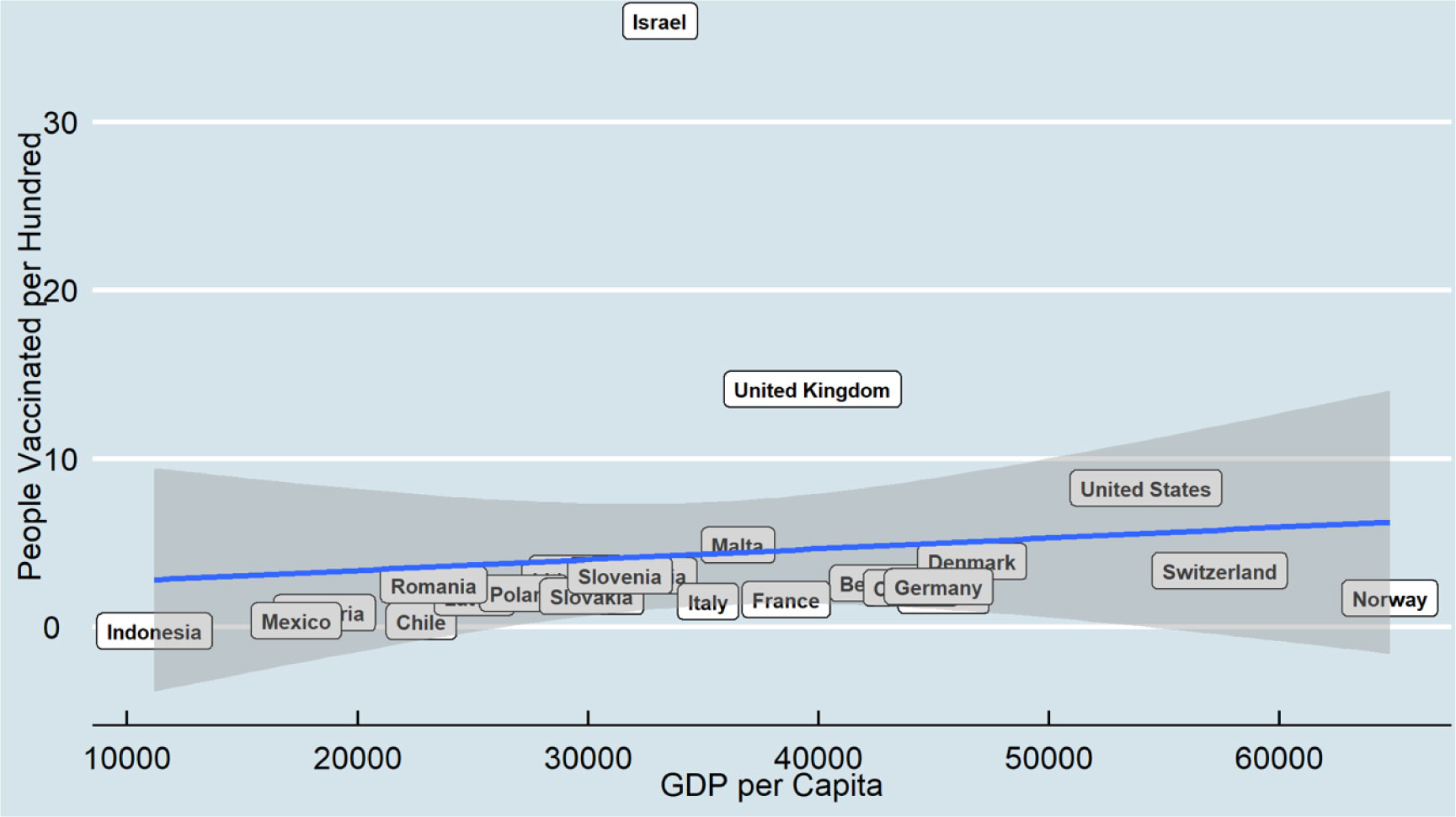
Since coronavirus disease 2019 (COVID-19) has continued to spread globally, many countries have started vaccinations at the end of December 2020. This research examines the relationship between COVID-19 vaccine distribution and two macro-socioeconomics measures, including human development index and gross domestic product, among 25 countries for two points in time, including February and August 2021. The COVID-19 dataset is a collection of the COVID-19 data maintained by Our World in Data. It is a daily updated dataset and includes confirmed cases, vaccinations, deaths, and testing data. Ordinary Least Squares was applied to examine how macro-socioeconomic measures predict the distribution of the COVID-19 vaccine over time.

Results
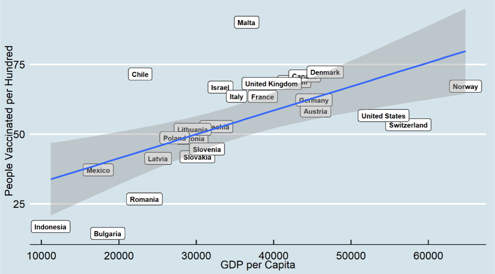
The results indicate that a higher gross domestic product per capita is positively associated with higher COVID-19 vaccine distribution, and this relationship becomes more robust over time. However, some countries may have more successful vaccine distribution results regardless of their gross domestic product. In addition, the result shows human development index does not have a significant relationship with vaccine distribution.

Conclusion
Economic measures may be counted as a more vital indicator for vaccine distribution as they have a more direct relationship distribution with health infrastructure than social measures such as human development index.
- COVID-19,
- immunization programs,
- vaccine distribution,
- gross domestic product,
- human development index,
- SARS-CoV-2 infection,
- Pfizer vaccine
Citation: Ali Roghani. The relationship between macro-socioeconomics determinants and COVID-19 vaccine distribution[J]. AIMS Public Health, 2021, 8(4): 655-664. doi: 10.3934/publichealth.2021052

Related Papers:

Abstract

Since coronavirus disease 2019 (COVID-19) has continued to spread globally, many countries have started vaccinations at the end of December 2020. This research examines the relationship between COVID-19 vaccine distribution and two macro-socioeconomics measures, including human development index and gross domestic product, among 25 countries for two points in time, including February and August 2021. The COVID-19 dataset is a collection of the COVID-19 data maintained by Our World in Data. It is a daily updated dataset and includes confirmed cases, vaccinations, deaths, and testing data. Ordinary Least Squares was applied to examine how macro-socioeconomic measures predict the distribution of the COVID-19 vaccine over time.

Results

The results indicate that a higher gross domestic product per capita is positively associated with higher COVID-19 vaccine distribution, and this relationship becomes more robust over time. However, some countries may have more successful vaccine distribution results regardless of their gross domestic product. In addition, the result shows human development index does not have a significant relationship with vaccine distribution.

Conclusion

Economic measures may be counted as a more vital indicator for vaccine distribution as they have a more direct relationship distribution with health infrastructure than social measures such as human development index.

Conflict of interest

The author declares no conflict of interest.

References

[1]	Agrawal G, Conway M, Heller J, et al. (2020) On pins and needles: Will COVID-19 vaccines save the world? Accessed November 24.
[2]	Coccia M (2021) Pandemic prevention: Lessons from COVID-19. Encyclopedia 1: 433-444. doi: 10.3390/encyclopedia1020036
[3]	Coccia M (2021) The relation between length of lockdown, numbers of infected people and deaths of Covid-19, and economic growth of countries: Lessons learned to cope with future pandemics similar to Covid-19 and to constrain the deterioration of economic system. Sci Total Environ 775: 145801. doi: 10.1016/j.scitotenv.2021.145801
[4]	Echoru I, Ajambo PD, Keirania E, et al. (2021) Sociodemographic factors associated with acceptance of COVID-19 vaccine and clinical trials in Uganda: a cross-sectional study in western Uganda. BMC Public Health 21: 1-8. doi: 10.1186/s12889-021-11197-7
[5]	Coccia M (2021) Preparedness of countries to face covid-19 pandemic crisis: Strategic positioning and underlying structural factors to support strategies of prevention of pandemic threats. Environ Res 203: 111678. doi: 10.1016/j.envres.2021.111678
[6]	Yuan J, Li M, Lv G, et al. (2020) Monitoring transmissibility and mortality of COVID-19 in Europe. Int J Infect Dis 95: 311-315. doi: 10.1016/j.ijid.2020.03.050
[7]	Coccia M (2020) An index to quantify environmental risk of exposure to future epidemics of the COVID-19 and similar viral agents: Theory and practice. Environ Res 191: 110155. doi: 10.1016/j.envres.2020.110155
[8]	Brett TS, Rohani P (2020) Transmission dynamics reveal the impracticality of COVID-19 herd immunity strategies. Pro Natl Acad Sci U S A 117: 25897-25903. doi: 10.1073/pnas.2008087117
[9]	Coccia M (2021) The effects of atmospheric stability with low wind speed and of air pollution on the accelerated transmission dynamics of COVID-19. Int J Environ Stud 78: 1-27. doi: 10.1080/00207233.2020.1802937
[10]	Coccia M (2020) How do low wind speeds and high levels of air pollution support the spread of COVID-19? Atmos Pollut Res 12: 437-445. doi: 10.1016/j.apr.2020.10.002
[11]	Candido DS, Claro IM, de Jesus JG, et al. (2020) Evolution and epidemic spread of SARS-CoV-2 in Brazil. Science 369: 1255-1260. doi: 10.1126/science.abd2161
[12]	Coccia M (2021) Effects of the spread of COVID-19 on public health of polluted cities: results of the first wave for explaining the dejà vu in the second wave of COVID-19 pandemic and epidemics of future vital agents. Environ Sci Pollut Res Int 28: 19147-19154. doi: 10.1007/s11356-020-11662-7
[13]	Domingo JL, Marquès M, Rovira J (2020) Influence of airborne transmission of SARS-CoV-2 on COVID-19 pandemic. A review. Environ Res 188: 109861. doi: 10.1016/j.envres.2020.109861
[14]	Frederiksen L, Zhang Y, Foged C, et al. (2020) The long road toward COVID-19 herd immunity: Vaccine Platform Technologies and Mass Immunization Strategies. Front Immunol 11: 1817. doi: 10.3389/fimmu.2020.01817
[15]	Mullard A (2020) How COVID-19 vaccines are being divided up around the world. Nature News .
[16]	Sheikh AB, Pal S, Javed N, et al. (2021) COVID-19 vaccination in developing nations: challenges and opportunities for innovation. Infect Dis Rep 13: 429-436. doi: 10.3390/idr13020041
[17]	Ghosh A, Nundy S, Mallick TK (2020) How India is dealing with COVID-19 pandemic. Sens Int 1: 100021. doi: 10.1016/j.sintl.2020.100021
[18]	Katz IT, Weintraub R, Bekker LG, et al. (2021) From vaccine nationalism to vaccine equity—Finding a path forward. N Engl J Med 384: 1281-1283. doi: 10.1056/NEJMp2103614
[19]	World Health Organization (2020) Health inequity and the effects of COVID-19: assessing, responding to and mitigating the socioeconomic impact on health to build a better future. World Health Organization. Regional Office for Europe No. WHO/EURO: 2020-1744-41495-56594.
[20]	Karmakar M, Lantz PM, Tipirneni R (2021) Association of social and demographic factors with COVID-19 incidence and death rates in the US. JAMA Netw Open 4: e2036462. doi: 10.1001/jamanetworkopen.2020.36462
[21]	Caspi G, Dayan A, Eshal Y, et al. (2021) Socioeconomic disparities and COVID-19 vaccination acceptance: a nationwide ecologic study. Clin Microbiol Infect S1198–743X(21)00277–9.
[22]	Qian Y, Fan W (2020) Who loses income during the COVID-19 outbreak? Evidence from China. Res Soc Strat Mobil 68: 100522.
[23]	Freed GL (2021) Actionable lessons for the US COVID vaccine program. Isr J Health Policy Res 10: 1-3. doi: 10.1186/s13584-021-00452-2
[24]	Schaffer DeRoo S, Pudalov NJ, Fu LY (2020) Planning for a COVID-19 vaccination program. JAMA 323: 2458-2459. doi: 10.1001/jama.2020.8711
[25]	Gutierrez FH (2017) Infant health during the 1980s peruvian crisis and long-term economic outcomes. World Dev 89: 71-87. doi: 10.1016/j.worlddev.2016.08.002
[26]	Shah A, Marks PW, Hahn SM (2020) Unwavering regulatory safeguards for COVID-19 vaccines. JAMA 324: 931-932. doi: 10.1001/jama.2020.15725
[27]	Ball P, Maxmen A (2020) The epic battle against coronavirus misinformation and conspiracy theories. Nature 581: 371-374. doi: 10.1038/d41586-020-01452-z
[28]	Dror AA, Eisenbach N, Taiber S, et al. (2020) Vaccine hesitancy: the next challenge in the fight against COVID-19. Eur J Epidemiol 35: 775-779. doi: 10.1007/s10654-020-00671-y
[29]	Stanton EA (2007) The human development index: A history. PERI Work Pap 85.
[30]	Viswanath K, Bekalu M, Dhawan D, et al. (2021) Individual and social determinants of COVID-19 vaccine uptake. BMC Public Health 21: 818. doi: 10.1186/s12889-021-10862-1
[31]	Harrison EA, Wu JW (2020) Vaccine confidence in the time of COVID-19. Eur J Epidemiol 35: 325-330. doi: 10.1007/s10654-020-00634-3
[32]	Our World in Data. Coronavirus Pandemic (COVID-19) Available from: https://ourworldindata.org/coronavirus.
[33]	World Bank Total population. Population, total-Least development countries: UN classification Available from: https://data.worldbank.org/indicator/SP.POP.TOTL?locations=XL.
[34]	World Bank GDP (constant 2010 US$) Available from: https://data.worldbank.org/indicator/NY.GDP.MKTP.KD.
[35]	Bloom DE, Canning D, Fink G (2014) Disease and development revisited. J Polit Econ 122: 1355-1366. doi: 10.1086/677189
[36]	Torjesen I (2021) Covid-19: Norway investigates 23 deaths in frail elderly patients after vaccination. BMJ 372: n149. doi: 10.1136/bmj.n149
[37]	Murphy J, Vallières F, Bentall RP, et al. (2021) Psychological characteristics associated with COVID-19 vaccine hesitancy and resistance in Ireland and the United Kingdom. Nat Commun 12: 29. doi: 10.1038/s41467-020-20226-9
[38]	Syed Alwi SAR, Rafidah E, Zurraini A, et al. (2021) A survey on COVID-19 vaccine acceptance and concern among Malaysians. BMC Public Health 21: 1129. doi: 10.1186/s12889-021-11071-6
[39]	Kanyike AM, Olum R, Kajjimu J, et al. (2021) Acceptance of the coronavirus disease-2019 vaccine among medical students in Uganda. Trop Med Health 49: 37. doi: 10.1186/s41182-021-00331-1
[40]	Schwarzinger M, Watson V, Arwidson P, et al. (2021) COVID-19 vaccine hesitancy in a representative working-age population in France: a survey experiment based on vaccine characteristics. Lancet Public Health 6: e210-e221. doi: 10.1016/S2468-2667(21)00012-8
[41]	Dooling K, McClung N, Chamberland M, et al. (2020) The advisory committee on immunization practices' interim recommendation for allocating initial supplies of COVID-19 vaccine-United States, 2020. MMWR Morb Mortal Wkly Rep 69: 1857-1859. doi: 10.15585/mmwr.mm6949e1
[42]	Elhadi M, Alsoufi A, Alhadi A, et al. (2021) Knowledge, attitude, and acceptance of healthcare workers and the public regarding the COVID-19 vaccine: a cross-sectional study. BMC Public Health 21: 955. doi: 10.1186/s12889-021-10987-3
[43]	Verger P, Peretti-Watel P (2021) Understanding the determinants of acceptance of COVID-19 vaccines: a challenge in a fast-moving situation. Lancet Public Health 6: e195-e196. doi: 10.1016/S2468-2667(21)00029-3
[44]	Wagner AL, Masters NB, Domek GJ, et al. (2019) Comparisons of vaccine hesitancy across five low- and middle-income countries. Vaccines 7: 155. doi: 10.3390/vaccines7040155
[45]	Mofijur M, Fattah I, Alam MA, et al. (2021) Impact of COVID-19 on the social, economic, environmental and energy domains: Lessons learnt from a global pandemic. Sustain Prod Consum 26: 343-359. doi: 10.1016/j.spc.2020.10.016
[46]	Coccia M (2020) Factors determining the diffusion of COVID-19 and suggested strategy to prevent future accelerated viral infectivity similar to COVID. Sci Total Environ 729: 138474. doi: 10.1016/j.scitotenv.2020.138474
[47]	Ghosh A, Nundy S, Ghosh S, et al. (2020) Study of COVID-19 pandemic in London (UK) from urban context. Cities 106: 102928. doi: 10.1016/j.cities.2020.102928
[48]	Roghani A, Panahi S (2021) Higher COVID-19 vaccination rates among unemployed in the United States: state level study in the first 100 days of vaccine initiation. medRxiv .

Reader Comments

Your name:*

Email:*
© 2021 the Author(s), licensee AIMS Press. This is an open access article distributed under the terms of the Creative Commons Attribution License (http://creativecommons.org/licenses/by/4.0)