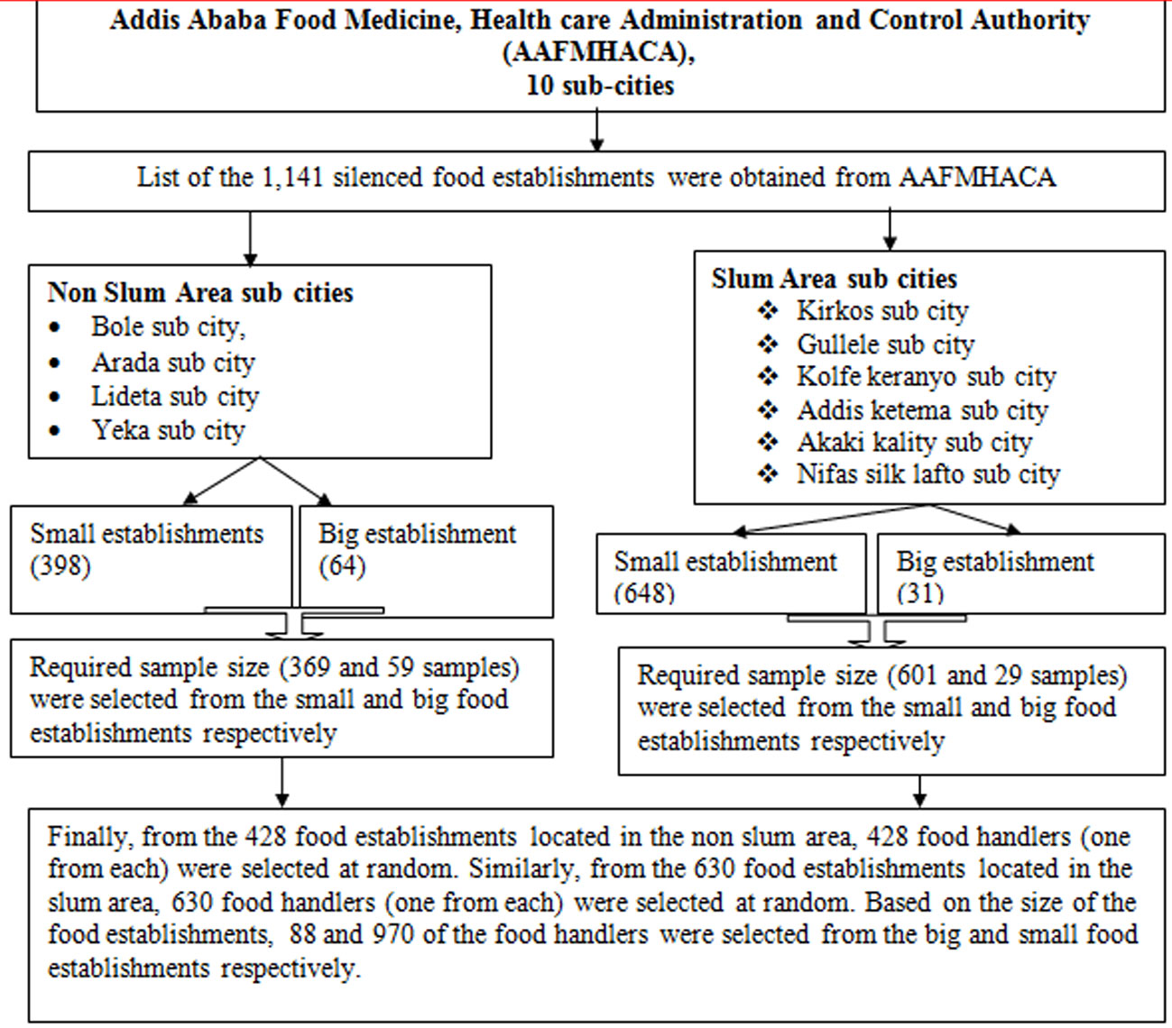
Introduction: Diarrheal diseases are threat everywhere, but its frequency and impact are more severe in developing countries. Diarrhea occurs world-wide and causes 4% of all deaths and 5% of health loss to disability. In 2016, it was the eighth leading cause of mortality. Moreover, data from the World Health Organization indicated that diarrheal diseases are causes for an estimated 2 million deaths annually. Therefore, this study aimed to assess diarrheal diseases and associated behavioural factors. Method: An institution based cross-sectional study was conducted. A stratified random sampling method was employed to select 1050 study participants. Participants were interviewed using structured questionnaire. To analysis the data, binary logistic regression and multivariable logistic regression analysis was conducted. Results: The two weeks prevalence of diarrhea was found to be 3.4%. Further, 1.6%, 10.5%, 10.7% and 9% of the food handlers had acute watery diarrhea, cough, an infection of runny nose and incidence of any fever respectively. Regular hand washing after toilet (AOR = 0.13 with 95% CI: 0.024, 0.72), using toilet while wearing protective clothes/gown (AOR = 5.39 with 95% CI; 1.59, 18.32), habit of eating raw beef and raw vegetables (AOR = 6.27 with 95% CI: 1.89–20.78), type of toilet (AOR = 4.07 with 95% CI: 0.29–6.67 were associated significantly with diarrhea. Conclusion: This assessment proved to be an essential activity for reduction of community diarrheal diseases, as a significant number of food handlers had diarrhea. Good sanitation, hygiene practice and a healthy lifestyle behavior can prevent diarrhea. A strong political commitment with appropriate budgetary allocation is essential for the control of diarrheal diseases.
Citation: Aderajew Mekonnen Girmay, Sirak Robele Gari, Bezatu Mengistie Alemu, Martin R. Evans, Azage Gebreyohannes Gebremariam. Diarrheal disease and associated behavioural factors among food handlers in Addis Ababa, Ethiopia[J]. AIMS Public Health, 2020, 7(1): 100-113. doi: 10.3934/publichealth.2020010
Introduction: Diarrheal diseases are threat everywhere, but its frequency and impact are more severe in developing countries. Diarrhea occurs world-wide and causes 4% of all deaths and 5% of health loss to disability. In 2016, it was the eighth leading cause of mortality. Moreover, data from the World Health Organization indicated that diarrheal diseases are causes for an estimated 2 million deaths annually. Therefore, this study aimed to assess diarrheal diseases and associated behavioural factors. Method: An institution based cross-sectional study was conducted. A stratified random sampling method was employed to select 1050 study participants. Participants were interviewed using structured questionnaire. To analysis the data, binary logistic regression and multivariable logistic regression analysis was conducted. Results: The two weeks prevalence of diarrhea was found to be 3.4%. Further, 1.6%, 10.5%, 10.7% and 9% of the food handlers had acute watery diarrhea, cough, an infection of runny nose and incidence of any fever respectively. Regular hand washing after toilet (AOR = 0.13 with 95% CI: 0.024, 0.72), using toilet while wearing protective clothes/gown (AOR = 5.39 with 95% CI; 1.59, 18.32), habit of eating raw beef and raw vegetables (AOR = 6.27 with 95% CI: 1.89–20.78), type of toilet (AOR = 4.07 with 95% CI: 0.29–6.67 were associated significantly with diarrhea. Conclusion: This assessment proved to be an essential activity for reduction of community diarrheal diseases, as a significant number of food handlers had diarrhea. Good sanitation, hygiene practice and a healthy lifestyle behavior can prevent diarrhea. A strong political commitment with appropriate budgetary allocation is essential for the control of diarrheal diseases.

| [1] |
Dagnew AB, Tewabe T, Miskir Y, et al. (2019) Prevalence of diarrhea and associated factors among under-five children in Bahir Dar city, Northwest Ethiopia: a cross-sectional study. BMC Infect Dis 19: 417. doi: 10.1186/s12879-019-4030-3

|
| [2] | (2015) World Health OrganizationWHO estimates of the global burden of foodborne diseases: foodborne disease burden epidemiology reference group 2007–2015. World Health Organization. |
| [3] | Ahmed T, Svennerholm A (2009) Diarrheal disease: Solutions to defeat a global killer. Path Catal Glob Health . |
| [4] |
Bbaale E (2011) Determinants of diarrhoea and acute respiratory infection among under-fives in Uganda. Australas Med J 4: 400-407. doi: 10.4066/AMJ.2011.723
|
| [5] |
Troeger C, Blacker BF, Khalil IA, et al. (2018) Estimates of the global, regional, and national morbidity, mortality, and aetiologies of diarrhoea in 195 countries: a systematic analysis for the Global Burden of Disease Study 2016. Lancet Infect Dis 18: 1211-1228. doi: 10.1016/S1473-3099(18)30362-1
|
| [6] |
Hodge J, Chang HH, Boisson S (2016) Assessing the Association between Thermotolerant Coliforms in Drinking Water and Diarrhea: An Analysis of Individual–Level Data from Multiple Studies. Environ Health Perspect 124: 1560-1567. doi: 10.1289/EHP156
|
| [7] | Williams P, Berkley J (2016) Severe acute malnutrition update: current WHO guidelines and the WHO essential medicine list for children. J Clin Pharmacol . |
| [8] | Jaffee S, Henson S, Unnevehr L, et al. (2018) World Health Organization Global Estimates and Regional Comparisons of the Burden of Foodborne Disease University of Southern California Los Angeles. |
| [9] |
Havelaar AH, Kirk MD, Torgerson PR, et al. (2015) World Health Organization global estimates and regional comparisons of the burden of foodborne disease. PLoS Med 12: e1001923. doi: 10.1371/journal.pmed.1001923
|
| [10] | Panchal PK, Bonhote P, Dworkin MS (2013) Food safety knowledge among restaurant food handlers in Neuchatel, Switzerland. Food Prot Trends 33: 133-144. |
| [11] | (2013) World Health OrganizationAdvancing food safety initiatives: strategic plan for food safety including foodborne zoonoses 2013–2022. World Health Organization. |
| [12] |
Sumner S, Brown LG, Frick R, et al. (2011) Factors associated with food workers working while experiencing vomiting or diarrhea. J Food Prot 74: 215-220. doi: 10.4315/0362-028X.JFP-10-108
|
| [13] | Waithaka PN, Maingi JM, Nyamache AK (2014) Physico-chemical and microbiological analysis in treated, stored and drinking water in Nakuru North, Kenya. |
| [14] | Grace D (2017) White paper Food safety in developing countries: research gaps and opportunities. Feed Future . |
| [15] |
Kotloff KL (2017) The burden and etiology of diarrheal illness in developing countries. Pediatr Clin North Am 64: 799-814. doi: 10.1016/j.pcl.2017.03.006
|
| [16] |
Ifeadike CO, Ironkwe OC, Adogu POU, et al. (2012) Prevalence and pattern of bacteria and intestinal parasites among food handlers in the Federal Capital Territory of Nigeria. Niger Med J 53: 166. doi: 10.4103/0300-1652.104389
|
| [17] |
Bain R, Cronk R, Hossain R, et al. (2014) Global assessment of exposure to faecal contamination through drinking water based on a systematic review. Trop Medi Int Health 19: 917-927. doi: 10.1111/tmi.12334
|
| [18] | World Health Organization (2014) Mortality and burden of disease from water and sanitation. Global Health Observatory (GHO) data. |
| [19] |
Girmay AM, Evans MR, Gari SR, et al. (2019) Urban health extension service utilization and associated factors in the community of Gullele sub-city administration, Addis Ababa, Ethiopia. Int J Community Med Public Health 6: 976-985. doi: 10.18203/2394-6040.ijcmph20190580
|
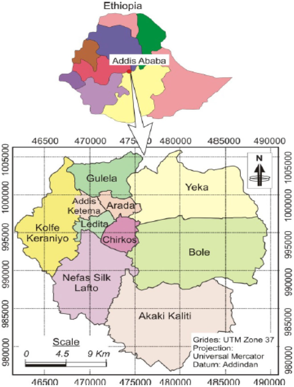
| [20] | Berhanu M, Raghuvanshi TK, Suryabhagavan KV (2017) Web-based GIS approach for tourism development in addis ababa city, Ethiopia. Malays J Remote Sens GIS 6: 13-25. |
| [21] |
Ma C, Wu S, Yang P, et al. (2014) Behavioural factors associated with diarrhea among adults over 18 years of age in Beijing, China. BMC Public Health 14: 451. doi: 10.1186/1471-2458-14-451
|
| [22] | Abera B, Biadegelgen F, Bezabih B (2010) Prevalence of Salmonella typhi and intestinal parasites among food handlers in Bahir Dar Town, Northwest Ethiopia. Ethiop J Health Dev 24. |
| [23] |
Llanes R, Somarriba L, Velázquez B, et al. (2016) Low prevalence of Vibrio cholerae O1 versus moderate prevalence of intestinal parasites in food-handlers working with health care personnel in Haiti. Pathog Global Health 110: 30-32. doi: 10.1080/20477724.2016.1141471
|
| [24] |
Scallan E, Majowicz SE, Hall G, et al. (2005) Prevalence of diarrhoea in the community in Australia, Canada, Ireland, and the United States. Int J Epidemiol 34: 454-460. doi: 10.1093/ije/dyh413
|
| [25] |
Mt S, Murugan S, Pm N, et al. (2014) Evaluation of hygienic and morbidity status of food handlers at eating establishment in coimbatore district, South India–An Empirical Study. Curr Res Nutr Food Sci J 2: 131-135. doi: 10.12944/CRNFSJ.2.3.04
|
| [26] | (2014) World Health OrganizationPreventing diarrhoea through better water, sanitation and hygiene: exposures and impacts in low-and middle-income countries. World Health Organization. |
Figures(2) / Tables(5)

Aderajew Mekonnen Girmay, Sirak Robele Gari, Bezatu Mengistie Alemu, Martin R. Evans, Azage Gebreyohannes Gebremariam. Diarrheal disease and associated behavioural factors among food handlers in Addis Ababa, Ethiopia[J]. AIMS Public Health, 2020, 7(1): 100-113. doi: 10.3934/publichealth.2020010


 DownLoad: