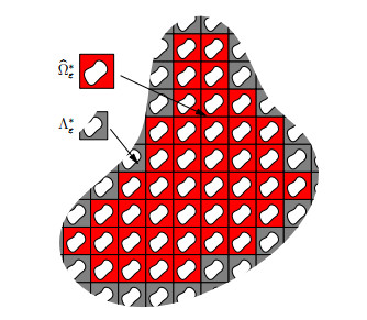
In this paper, we consider a class of elliptic problems in a periodically perforated domain with $ L^1 $ data and nonlinear Robin conditions on the boundary of the holes. Using the framework of renormalized solutions, which is well adapted to this situation, we show a convergence result for the truncated energy in the quasilinear case. When the operator is linear, we also prove a corrector result. Since we cannot expect to have solutions belonging to $ H^1 $, the main difficulty is to express the corrector result through the truncations of the solutions, together with the fact that the definition of a renormalized solution contains test functions which are nonlinear functions of the solution itself.
Citation: Patrizia Donato, Olivier Guibé, Alip Oropeza. Corrector results for a class of elliptic problems with nonlinear Robin conditions and $ L^1 $ data[J]. Networks and Heterogeneous Media, 2023, 18(3): 1236-1259. doi: 10.3934/nhm.2023054
In this paper, we consider a class of elliptic problems in a periodically perforated domain with $ L^1 $ data and nonlinear Robin conditions on the boundary of the holes. Using the framework of renormalized solutions, which is well adapted to this situation, we show a convergence result for the truncated energy in the quasilinear case. When the operator is linear, we also prove a corrector result. Since we cannot expect to have solutions belonging to $ H^1 $, the main difficulty is to express the corrector result through the truncations of the solutions, together with the fact that the definition of a renormalized solution contains test functions which are nonlinear functions of the solution itself.

| [1] |
M. Artola, G. Duvaut, Un résultat d'homogénéisation pour une classe de problèmes de diffusion non linéaires stationnaires, Ann. Fac. Sci. Toulouse Math., 4 (1982), 1–28. https://doi.org/10.5802/afst.572 doi: 10.5802/afst.572

|
| [2] | P. Bénilan, L. Boccardo, T. Gallouët, R. Gariepy, M. Pierre, J. L. Vazquez, An $L^ 1$-theory of existence and uniqueness of solutions of nonlinear elliptic equations, Ann. Sc. Norm. Super. Pisa Cl. Sci., 22 (1995), 241–273. https://eudml.org/doc/84205 |
| [3] | G. Papanicolau, A. Bensoussan, J. L. Lions, Studies in Mathematics and its Applications, Asymptotic Analysis for Periodic Structures. Amsterdam: Elsevier, 1978. |
| [4] |
D. Cioranescu, A. Damlamian, P. Donato, G. Griso, R. Zaki, The periodic unfolding method in domains with holes, SIAM J. Math. Anal., 44 (2012), 718–760. https://doi.org/10.1137/100817942 doi: 10.1137/100817942
|
| [5] |
D. Cioranescu, A. Damlamian, G. Griso, Periodic unfolding and homogenization, C. R. Math., 335 (2022), 99–104. https://doi.org/10.1016/S1631-073X(02)02429-9 doi: 10.1016/S1631-073X(02)02429-9
|
| [6] |
D. Cioranescu, A. Damlamian, G. Griso, The periodic unfolding method in homogenization, SIAM J. Math. Anal., 40 (2008), 1585–1620. https//doi.org/10.1137/080713148 doi: 10.1137/080713148
|
| [7] | D. Cioranescu, A. Damlamian, G. Griso, The Periodic Unfolding Method, Theory and Applications to Partial Differential Problems, Singapore: Springer, 2018. https//doi.org/10.1007/978-981-13-3032-2 |
| [8] | D. Cioranescu, P. Donato, An Introduction to Homogenization, Oxford: Oxford University Press, 1999. |
| [9] | G. Dal Maso, F. Murat, L. Orsina, A. Prignet, Renormalized solutions of elliptic equations with general measure data, Ann. Sc. Norm. Super. Pisa, Cl. Sci., IV. Ser., 28 (1999), 741–808. https://eudml.org/doc/84396 |
| [10] | P. Donato, A. Gaudiello, L. Sgambati, Homogenization of bounded solutions of elliptic equations with quadratic growth in periodically perforated domains, Asymptotic Anal., 16 (1998), 223–243. |
| [11] |
P. Donato, O. Guibé, A. Oropeza, Homogenization of quasilinear elliptic problems with nonlinear Robin conditions and $L^1$ data, J. Math. Pures Appl., 120 (2018), 91–129. https//doi.org/10.1016/j.matpur.2017.10.002 doi: 10.1016/j.matpur.2017.10.002
|
| [12] |
O. Guibé, A. Oropeza, Renormalized solutions of elliptic equations with Robin boundary conditions, Acta Math. Sci., 37 (2017), 889–910. https//doi.org/10.1016/S0252-9602(17)30046-2 doi: 10.1016/S0252-9602(17)30046-2
|
Figures(4)
Patrizia Donato, Olivier Guibé, Alip Oropeza. Corrector results for a class of elliptic problems with nonlinear Robin conditions and $ L^1 $ data[J]. Networks and Heterogeneous Media, 2023, 18(3): 1236-1259. doi: 10.3934/nhm.2023054


 DownLoad: