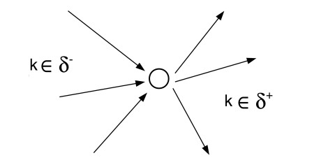
We discuss coupling conditions for the p-system in case of a transition from supersonic states to subsonic states. A single junction with adjacent pipes is considered where on each pipe the gas flow is governed by a general p-system. By extending the notion of demand and supply known from traffic flow analysis we obtain a constructive existence result of solutions compatible with the introduced conditions.
Citation: Martin Gugat, Michael Herty, Siegfried Müller. Coupling conditions for the transition from supersonic to subsonic fluid states[J]. Networks and Heterogeneous Media, 2017, 12(3): 371-380. doi: 10.3934/nhm.2017016
We discuss coupling conditions for the p-system in case of a transition from supersonic states to subsonic states. A single junction with adjacent pipes is considered where on each pipe the gas flow is governed by a general p-system. By extending the notion of demand and supply known from traffic flow analysis we obtain a constructive existence result of solutions compatible with the introduced conditions.

| [1] |
Coupling conditions for gas networks governed by the isothermal Euler equations. Netw. Heterog. Media (2006) 1: 295-314 (electronic). 
|
| [2] |
Gas flow in pipeline networks. Netw. Heterog. Media (2006) 1: 41-56.
|
| [3] | A. Bressan, Hyperbolic Systems of Conservation Laws, The One-Dimensional Cauchy Problem, Oxford Lecture Series in Mathematics and its Applications, 20, Oxford University Press, Oxford, 2000. |
| [4] |
Flow on networks: recent results and perspectives. European Mathematical Society-Surveys in Mathematical Sciences (2014) 1: 47-111.
|
| [5] |
The Cauchy problem for the Euler equations for compressible fluids. Handbook of Mathematical Fluid Dynamics (2002) 1: 421-543.
|
| [6] |
Traffic flow on a road network. SIAM J. Math. Anal. (2005) 36: 1862-1886 (electronic).
|
| [7] |
Optimal control in networks of pipes and canals. SIAM J. Control Optim. (2009) 48: 2032-2050.
|
| [8] |
A well posed Riemann problem for the p-system at a junction. Netw. Heterog. Media (2006) 1: 495-511.
|
| [9] |
On the Cauchy problem for the p-system at a junction. SIAM J. Math. Anal. (2008) 39: 1456-1471.
|
| [10] |
On 2×2 conservation laws at a junction. SIAM J. Math. Anal. (2008) 40: 605-622.
|
| [11] | Thèorie du mouvement non-permanent des eaux, avec application aux crues des rivière at à l'introduction des marèes dans leur lit.. C.R. Acad. Sci. Paris (1871) 73: 147-154. |
| [12] | M. Garavello and B. Piccoli, Traffic Flow on Networks, vol. 1 of AIMS Series on Applied Mathematics, American Institute of Mathematical Sciences (AIMS), Springfield, MO, 2006, Conservation laws models. |
| [13] |
E. Godlewski and P. -A. Raviart,
Numerical Approximation of Hyperbolic Systems of Conservation Laws, Applied Mathematical Sciences, 118, Springer-Verlag, New York, 1996. doi: 10.1007/978-1-4612-0713-9
|
| [14] |
Coupling conditions for a class of second-order models for traffic flow. SIAM J. Math. Anal. (2006) 38: 595-616.
|
| [15] |
Assessment of coupling conditions in water way intersections. Internat. J. Numer. Methods Fluids (2013) 71: 1438-1460.
|
| [16] |
A mathematical model of traffic flow on a network of unidirectional roads. SIAM J. Math. Anal. (1995) 26: 999-1017.
|
| [17] |
Riemann problems with a kink. SIAM J. Math. Anal. (1999) 30: 497-515 (electronic).
|
| [18] | S. Joana, M. Joris and T. Evangelos, Technical and Economical Characteristics of Co2 Transmission Pipeline Infrastructure, Technical report, JRC Scientic and Technical Reports, European Commission. |
| [19] | Les modeles macroscopiques du traffic. Annales des Ponts. (1993) 67: 24-45. |
| [20] |
Experimental assessment of scale effects affecting two-phase flow properties in hydraulic jumps. Experiments in Fluids (2008) 45: 513-521.
|
| [21] |
Simulation of transient flow in gas networks. Int. Journal for Numerical Methods in Fluid Dynamics (1984) 4: 13-23.
|
| [22] | B. Sultanian, Fluid Mechanics: An Intermediate Approach, CRC Press, 2015. |
| [23] |
R. Ugarelli and V. D. Federico, Transition from supercritical to subcritical regime in free surface flow of yield stress fluids Geophys. Res. Lett. , 34 (2007), L21402. doi: 10.1029/2007GL031487
|


Figures(3) / Tables(2)
Martin Gugat, Michael Herty, Siegfried Müller. Coupling conditions for the transition from supersonic to subsonic fluid states[J]. Networks and Heterogeneous Media, 2017, 12(3): 371-380. doi: 10.3934/nhm.2017016


 DownLoad: