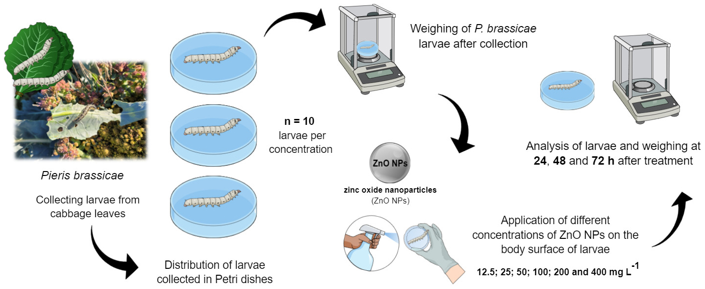
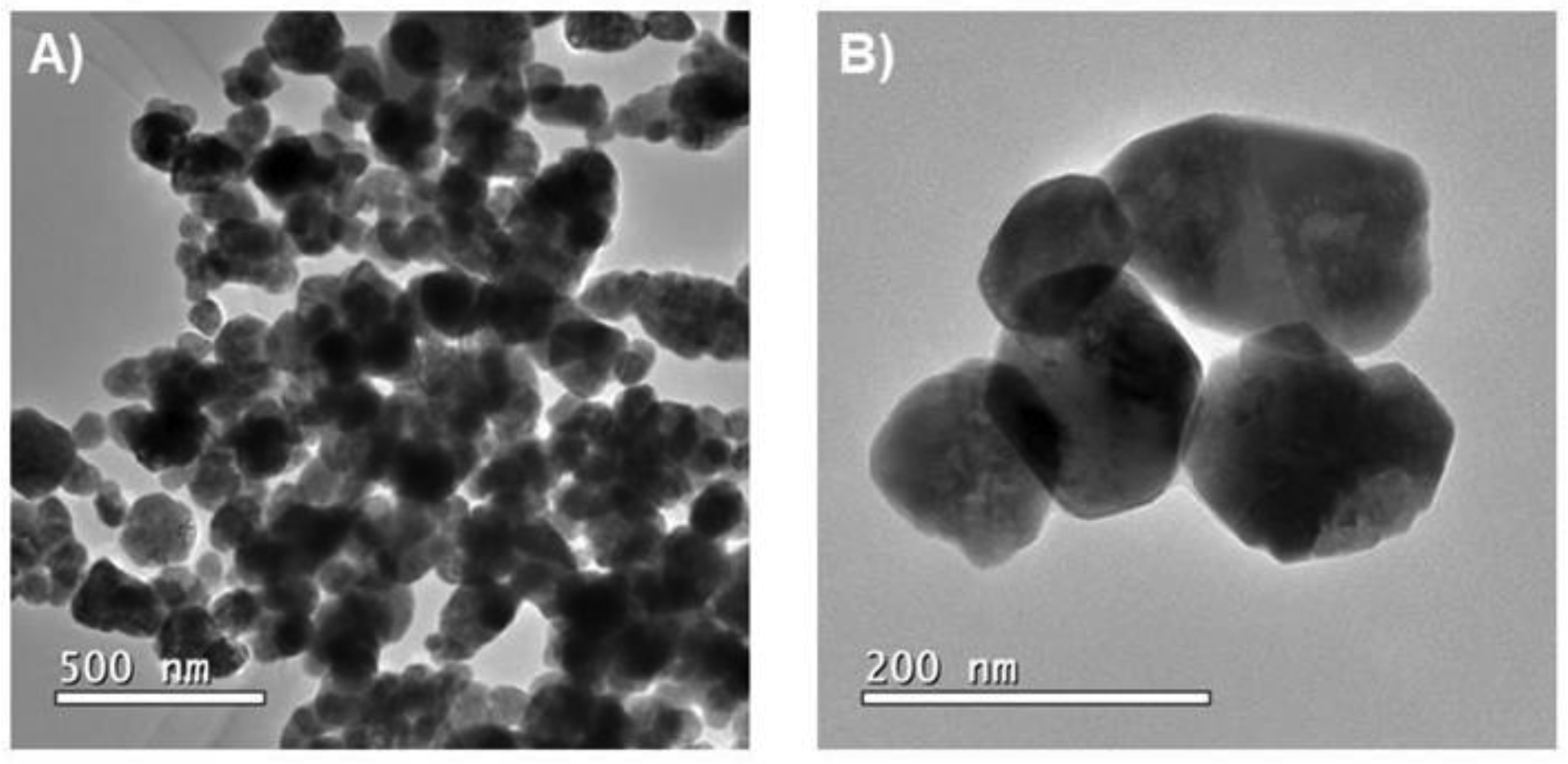
Pieris brassicae is commonly known as the cabbage moth and is a species known to be invasive, thereby causing serious damage to vegetables and subsequently leading to total crop loss. Formulations of nanopesticides can provide unique characteristics such as size and shape, in addition to having integrated properties in a single material, making them efficient in pest management and protection against diseases in a single material; it can be applied in small volumes, with a greater precision, lower input costs, and a potential reduction in environmental contamination. Nanotechnology is a type of alternative and highly effective technology in several sectors, mainly in agriculture and the enrichment and fortification of cultivars. Hydrothermal synthesis is a type of process used to obtain nanoparticles with a more uniform crystallinity and aging of nanocrystallites, where high temperatures and pressures help to reduce particle aggregation. Chemically synthesized metal nanoparticles, such as zinc oxide nanoparticles (ZnO NPs), can find wide applications and success against different types of pests, such as larvae. The present study focuses on the application of different concentrations of ZnO NPs (12.5, 25, 50, 100, 200 and 400 mg/L) on the body surface of P. brassicae to verify their possible pesticide activity against these larvae. The results of this study suggest a non-intuitive pesticidal activity of ZnO NPs against cabbage moth larvae. The highest mortality percentage of larvae against the treatments occurred at the concentration of 200 mg/L of ZnO NPs, represented by a rate of 100% in the 72-h period of the experiment. Finally, the results of the present study with ZnO NPs and P. brassicae larvae suggest an initial trigger for future possibilities of exploration and more in-depth studies to clarify the interaction of ZnO NPs and the possible metabolic pathways triggered in these insect pests.
Citation: Isabella Martins Lourenço, Amedea Barozzi Seabra, Marcelo Lizama Vera, Nicolás Hoffmann, Olga Rubilar Araneda, Leonardo Bardehle Parra. Synthesis and application of zinc oxide nanoparticles in Pieris brassicae larvae as a possible pesticide effect[J]. AIMS Molecular Science, 2024, 11(4): 351-366. doi: 10.3934/molsci.2024021
Pieris brassicae is commonly known as the cabbage moth and is a species known to be invasive, thereby causing serious damage to vegetables and subsequently leading to total crop loss. Formulations of nanopesticides can provide unique characteristics such as size and shape, in addition to having integrated properties in a single material, making them efficient in pest management and protection against diseases in a single material; it can be applied in small volumes, with a greater precision, lower input costs, and a potential reduction in environmental contamination. Nanotechnology is a type of alternative and highly effective technology in several sectors, mainly in agriculture and the enrichment and fortification of cultivars. Hydrothermal synthesis is a type of process used to obtain nanoparticles with a more uniform crystallinity and aging of nanocrystallites, where high temperatures and pressures help to reduce particle aggregation. Chemically synthesized metal nanoparticles, such as zinc oxide nanoparticles (ZnO NPs), can find wide applications and success against different types of pests, such as larvae. The present study focuses on the application of different concentrations of ZnO NPs (12.5, 25, 50, 100, 200 and 400 mg/L) on the body surface of P. brassicae to verify their possible pesticide activity against these larvae. The results of this study suggest a non-intuitive pesticidal activity of ZnO NPs against cabbage moth larvae. The highest mortality percentage of larvae against the treatments occurred at the concentration of 200 mg/L of ZnO NPs, represented by a rate of 100% in the 72-h period of the experiment. Finally, the results of the present study with ZnO NPs and P. brassicae larvae suggest an initial trigger for future possibilities of exploration and more in-depth studies to clarify the interaction of ZnO NPs and the possible metabolic pathways triggered in these insect pests.

| [1] | Klingshirn CF, Meyer BK, Waag A, et al. (2010) Zinc oxide: From fundamental properties towards novel applications. Berlin, Heidelberg: Springer. https://doi.org/10.1007/978-3-642-10577-7 |
| [2] | Espitia PJP, Otoni CG, Soares NFF (2016) Zinc oxide nanoparticles for food packaging applications. Antimicrobial food packaging . Cambridge, MA, USA: Academic Press 425-431. https://doi.org/10.1016/B978-0-12-800723-5.00034-6 |
| [3] | Alves Z, Ferreira NM, Figueiredo G, et al. (2022) Electrically conductive and antimicrobial agro-food waste biochar functionalized with zinc oxide particles. Int J Mol Sci 23: 8022. https://doi.org/10.3390/ijms23148022 |
| [4] | Taheri M, Qarache HA, Qarache AA, et al. (2015) The effects of zinc-oxide nanoparticles on growth parameters of corn (SC704). STEM Fellowship J 1: 17-20. https://doi.org/10.17975/sfj-2015-011 |
| [5] | Abdallah Y, Liu M, Ogunyemi SO, et al. (2020) Bioinspired green synthesis of chitosan and zinc oxide nanoparticles with strong antibacterial activity against rice pathogen Xanthomonas oryzae pv. oryzae. Molecules 25: 4795. https://doi.org/10.3390/molecules25204795 |
| [6] | Thounaojam TC, Meetei TT, Devi YB, et al. (2021) Zinc oxide nanoparticles (ZnO-NPs): A promising nanoparticle in renovating plant science. Acta Physiol Plant 43: 136. https://doi.org/10.1007/s11738-021-03307-0 |
| [7] | Wang X, Yang X, Chen S, et al. (2016) Zinc oxide nanoparticles affect biomass accumulation and photosynthesis in Arabidopsis. Front Plant Sci 6: 1243. https://doi.org/10.3389/fpls.2015.01243 |
| [8] | Zoufan P, Baroonian M, Zargar B (2020) ZnO nanoparticles-induced oxidative stress in Chenopodium murale L, Zn uptake, and accumulation under hydroponic culture. Environ Sci Pollut Res 27: 11066-11078. https://doi.org/10.1007/s11356-020-07735-2 |
| [9] | Pokhrel LR, Dubey B (2013) Evaluation of developmental responses of two crop plants exposed to silver and zinc oxide nanoparticles. Sci Total Environ 452: 321-332. https://doi.org/10.1016/j.scitotenv.2013.02.059 |
| [10] | Zhu J, Wang J, Zhan X, et al. (2021) Role of charge and size in the translocation and distribution of zinc oxide particles in wheat cells. ACS Sustain Chem Eng 9: 11556-11564. https://doi.org/10.1021/acssuschemeng.1c04080 |
| [11] | Hameed RS, Hassan ZN, Shafeeq MAA (2022) Bioactivity of insecticides nanoparticles for pest control: Review. Nat J Pharm Sci 2: 17-23. https://doi.org/10.22271/27889262.2022.v2.i1a.31 |
| [12] | Zhang L, Yan C, Guo Q, et al. (2018) The impact of agricultural chemical inputs on environment: Global evidence from informetrics analysis and visualization. Int J Low-Carbon Technol 13: 338-352. https://doi.org/10.1093/ijlct/cty039 |
| [13] | Fincheira P, Hoffmann N, Tortella G, et al. (2023) Eco-efficient systems based on nanocarriers for the controlled release of fertilizers and pesticides: Toward smart agriculture. Nanomaterials 13: 1978. https://doi.org/10.3390/nano13131978 |
| [14] | Kumar A, Choudhary A, Kaur H, et al. (2021) Smart nanomaterial and nanocomposite with advanced agrochemical activities. Nanoscale Res Lett 16: 156. https://doi.org/10.1186/s11671-021-03612-0 |
| [15] | Del Prado-Lu JL (2015) Insecticide residues in soil, water, and eggplant fruits and farmers' health effects due to exposure to pesticides. Environ Health Prev Med 20: 53-62. https://doi.org/10.1007/s12199-014-0425-3 |
| [16] | Aktar W, Sengupta D, Chowdhury A (2009) Impact of pesticides use in agriculture: their benefits and hazards. Interdiscip Toxicol 2: 1-12. https://doi.org/10.2478/v10102-009-0001-7 |
| [17] | Sahoo D, Mandal A, Mitra T, et al. (2018) Nanosensing of pesticides by zinc oxide quantum dot: An optical and electrochemical approach for the detection of pesticides in water. J Agric Food Chem 66: 414-423. https://doi.org/10.1021/acs.jafc.7b04188 |
| [18] | Chen H, Seiber JN, Hotze M (2014) ACS select on nanotechnology in food and agriculture: A perspective on implications and applications. J Agric Food Chem 62: 1209-1212. https://doi.org/10.1021/jf5002588 |
| [19] | Kaur A, Bhatt DP, Raja L (2022) Applications of nanotechnology in agriculture, with a focus on insect pest management. NanoWorld J 8: S76-S82. https://doi.org/10.17756/nwj.2022-s1-015 |
| [20] | Sahayaraj K (2014) Nanotechnology and plant biopesticides: An overview. Advances in plant biopesticides . New Delhi: Springer 279-293. https://doi.org/10.1007/978-81-322-2006-0_14 |
| [21] | Stadler T, Buteler M, Weaver DK (2010) Novel use of nanostructured alumina as an insecticide. Pest Manag Sci 66: 577-579. https://doi.org/10.1002/ps.1915 |
| [22] | He L, Liu Y, Mustapha A, et al. (2011) Antifungal activity of zinc oxide nanoparticles against Botrytis cinerea and Penicillium expansum. Microbiol Res 166: 207-215. https://doi.org/10.1016/j.micres.2010.03.003 |
| [23] | Vijayakumar S, Vinoj G, Malaikozhundan B, et al. (2015) Plectranthus amboinicus leaf extract mediated synthesis of zinc oxide nanoparticles and its control of methicillin resistant Staphylococcus aureus biofilm and blood sucking mosquito larvae. Spectrochim Acta A 137: 886-891. https://doi.org/10.1016/j.saa.2014.08.064 |
| [24] | Roopan SM, Mathew RS, Mahesh SS, et al. (2019) Environmental friendly synthesis of zinc oxide nanoparticles and estimation of its larvicidal activity against Aedes aegypti. Int J Environ Sci Technol 16: 8053-8060. https://doi.org/10.1007/s13762-018-2175-z |
| [25] | Hasan F, Ansari MS (2011) Effects of different brassicaceous host plants on the fitness of Pieris brassicae (L.). Crop Prot 30: 854-862. https://doi.org/10.1016/j.cropro.2011.02.024 |
| [26] | Chahil GS, Kular JS (2013) Biology of Pieris brassicae (Linn.) on different Brassica species in the plains of Punjab. J Plant Prot Res 53: 53-59. |
| [27] | Ali S, Ullah MI, Arshad M, et al. (2017) Effect of botanicals and synthetic insecticides on Pieris brassicae (L., 1758) (Lepidoptera: Pieridae). Turk Entomol Derg 41: 275-284. https://doi.org/10.16970/entoted.308941 |
| [28] | Mazurkiewicz A, Tumialis D, Pezowicz E, et al. (2017) Sensitivity of Pieris brassicae, P. napi and P. rapae (Lepidoptera: Pieridae) larvae to native strains of Steinernema feltiae (Filipjev, 1934). J Plant Dis Prot 124: 521-524. https://doi.org/10.1007/s41348-017-0118-4 |
| [29] | Karnavar GK (1983) Studies on the population control of Pieris brassicae L. by Apanteles glomeratus L. Int J Trop Insect Sci 4: 397-399. https://doi.org/10.1017/S1742758400002460 |
| [30] | Montezano DG, Specht A, Sosa-Gomez DR, et al. (2016) Host plants of Spodoptera frugiperda (Lepidoptera: Noctuidae) in the Americas. Afr Entomol 26: 286-300. https://doi.org/10.4001/003.026.0286 |
| [31] | Pittarate S, Rajula J, Rahman A, et al. (2021) Insecticidal effect of zinc oxide nanoparticles against Spodoptera frugiperda under laboratory conditions. Insects 12: 1017. https://doi.org/10.3390/insects12111017 |
| [32] | Pittarate S, Perumal V, Kannan S, et al. (2023) Insecticidal efficacy of nanoparticles against Spodoptera frugiperda (J.E. Smith) larvae and their impact in the soil. Heliyon 9: e16133. https://doi.org/10.1016/j.heliyon.2023.e16133 |
| [33] | Debnath N, Das S, Seth D, et al. (2011) Entomotoxic effect of silica nanoparticles against Sitophilus oryzae (L.). J Pest Sci 84: 99-105. https://doi.org/10.1007/s10340-010-0332-3 |
| [34] | Murugan K, Wei J, Alsalhi MS, et al. (2017) Magnetic nanoparticles are highly toxic to chloroquine-resistant Plasmodium falciparum, dengue virus (DEN-2), and their mosquito vectors. Parasitol Res 116: 495-502. https://doi.org/10.1007/s00436-016-5310-0 |
| [35] | Raju IM, Rao TS, Lakshmi KVD, et al. (2019) Poly 3-Thenoic acid sensitized, copper doped anatase/brookite TiO2 nanohybrids for enhanced photocatalytic degradation of an organophosphorus pesticide. J Environ Chem Eng 7: 103211. https://doi.org/10.1016/j.jece.2019.103211 |
| [36] | Tunçsoy BS (2018) Toxicity of nanoparticles on insects: A review. Adana Sci Technol Univ 1: 49-61. |
| [37] | Khan M, Khan MAS, Borah KK, et al. (2021) The potential exposure and hazards of metal-based nanoparticles on plants and environment, with special emphasis on ZnO NPs, TiO2 NPs, and AgNPs: A review. Environ Adv 6: 100128. https://doi.org/10.1016/j.envadv.2021.100128 |
| [38] | Rai M, Kon K, Ingle A, et al. (2014) Broad-spectrum bioactivities of silver nanoparticles: The emerging trends and future prospects. Appl Microbiol Biotechnol 98: 1951-1961. https://doi.org/10.1007/s00253-013-5473-x |
| [39] | Yasur J, Pathipati UR (2015) Lepidopteran insect susceptibility to silver nanoparticles and measurement of changes in their growth, development and physiology. Chemosphere 124: 92-102. https://doi.org/10.1016/j.chemosphere.2014.11.029 |
| [40] | Mao BH, Chen ZY, Wang YJ, et al. (2018) Silver nanoparticles have lethal and sublethal adverse effects on development and longevity by inducing ROS-mediated stress responses. Sci Rep 8: 2445. https://doi.org/10.1038/s41598-018-20728-z |
| [41] | Lourenço IM, Freire BM, Pieretti JC, et al. (2023) Implications of ZnO nanoparticles and S-Nitrosoglutathione on nitric oxide, Reactive oxidative species, photosynthetic pigments, and ionomic profile in rice. Antioxidants 12: 1871. https://doi.org/10.3390/antiox12101871 |
| [42] | Madathil ANP, Vanaja KA, Jayaraj MK (2007) Synthesis of ZnO nanoparticles by hydrothermal method. Nanophotonic Mater IV 6639: 47-55. https://doi.org/10.1117/12.730364 |
| [43] | Ismail AA, El-Midany A, Abdel-Aal EA, et al. (2005) Application of statistical design to optimize the preparation of ZnO nanoparticles via hydrothermal technique. Mater Lett 59: 1924-1928. https://doi.org/10.1016/j.matlet.2005.02.027 |
| [44] | Rai P, Yu YT (2012) Citrate-assisted hydrothermal synthesis of single crystalline ZnO nanoparticles for gas sensor application. Sensor Actuat B-Chem 173: 58-65. https://doi.org/10.1016/j.snb.2012.05.068 |
| [45] | Vlazan P, Ursu DH, Irina-Moisescu C, et al. (2015) Structural and electrical properties of TiO2/ZnO core–shell nanoparticles synthesized by hydrothermal method. Mater Charact 101: 153-158. https://doi.org/10.1016/j.matchar.2015.01.017 |
| [46] | Benelli G (2018) Mode of action of nanoparticles against insects. Environ Sci Pollut Res 25: 12329-12341. https://doi.org/10.1007/s11356-018-1850-4 |
| [47] | Jiang X, Miclăuş T, Wang L, et al. (2015) Fast intracellular dissolution and persistent cellular uptake of silver nanoparticles in CHO-K1 cells: Implication for cytotoxicity. Nanotoxicology 9: 181-189. https://doi.org/10.3109/17435390.2014.907457 |
| [48] | Rai M, Kon K, Ingle A, et al. (2014) Broad-spectrum bioactivities of silver nanoparticles: The emerging trends and future prospects. Appl Microbiol Biotechnol 98: 1951-1961. https://doi.org/10.1007/s00253-013-5473-x |
| [49] | Peng YH, Tso CP, Tsai YC, et al. (2015) The effect of electrolytes on the aggregation kinetics of three different ZnO nanoparticles in water. Sci Total Environ 530–531: 183-190. https://doi.org/10.1016/j.scitotenv.2015.05.059 |
| [50] | Fouda A, Hassan SED, Salem SS, et al. (2018) In-vitro cytotoxicity, antibacterial, and UV protection properties of the biosynthesized Zinc oxide nanoparticles for medical textile applications. Microb Pathogenesis 125: 252-261. https://doi.org/10.1016/j.micpath.2018.09.030 |
| [51] | Hoffmann N, Tortella G, Hermosilla E, et al. (2022) Comparative toxicity assessment of eco-friendly synthesized superparamagnetic iron oxide nanoparticles (SPIONs) in plants and aquatic model organisms. Minerals 12: 451. https://doi.org/10.3390/min12040451 |
| [52] | Abd El-Wahab RA, Anwar EM (2014) The effect of direct and indirect use of nanoparticles on cotton leaf worm, Spodoptera littoralis. Int J Biol Sci 1: 17-24. |
| [53] | Fouda A, Hassan SE, Salem SS, et al. (2018) In-vitro cytotoxicity, antibacterial, and UV protection properties of the biosynthesized zinc oxide nanoparticles for medical textile applications. Microb Pathogenesis 125: 252-261. https://doi.org/10.1016/j.micpath.2018.09.030 |
| [54] | Eskin A, Nurullahoğlu ZU (2022) Effect of zinc oxide nanoparticles (ZnO NPs) on the biology of Galleria mellonella L. (Lepidoptera: Pyralidae). J Basic Appl Zool 83: 54. https://doi.org/10.1186/s41936-022-00318-2 |
| [55] | Grisakova M, Metspalu L, Jõgar K, et al. (2006) Effects of biopesticide Neem EC on the large white butterfly, Pieris brassicae L. (Lepidoptera, Pieridae). Agron Res 4: 181-186. |
| [56] | Thakur P, Thakur S, Kumari P, et al. (2022) Nano-insecticide: Synthesis, characterization, and evaluation of insecticidal activity of ZnO NPs against Spodoptera litura and Macrosiphum euphorbiae. Appl Nanosci 12: 3835-3850. https://doi.org/10.1007/s13204-022-02530-6 |
| [57] | Asghar MS, Sarwar ZM, Almadiy AA, et al. (2022) Toxicological effects of silver and zinc oxide nanoparticles on the biological and life table parameters of Helicoverpa armigera (Noctuidae: Lepidoptera). Agriculture 12: 1744. https://doi.org/10.3390/agriculture12101744 |
| [58] | Alian RS, Dziewiecka M, Kedziorski A (2021) Do nanoparticles cause hormesis? Early physiological compensatory response in house crickets to a dietary admixture of GO, Ag, and GOAg composite. Sci Total Environ 788: 147801. https://doi.org/10.1016/j.scitotenv.2021.147801 |
| [59] | Agathokleous E, Araminiene V, Belz RG, et al. (2019) A quantitative assessment of hormetic responses of plants to ozone. Environ Res 176: 108527. https://doi.org/10.1016/j.envres.2019.108527 |


Figures(3) / Tables(1)

Isabella Martins Lourenço, Amedea Barozzi Seabra, Marcelo Lizama Vera, Nicolás Hoffmann, Olga Rubilar Araneda, Leonardo Bardehle Parra. Synthesis and application of zinc oxide nanoparticles in Pieris brassicae larvae as a possible pesticide effect[J]. AIMS Molecular Science, 2024, 11(4): 351-366. doi: 10.3934/molsci.2024021


 DownLoad: