This paper is devoted to the mathematical analysis of the contact capabilities of the fluid-structure interaction (FSI) model with seepage reported in [Comput. Methods Appl. Mech., 392:114637, 2022]. In the case of a rigid disk moving over a fixed horizontal plane, we show that this model encompasses contact and hence removes the non collision paradox of traditional FSI models which rely on Dirichlet or Dirichlet/Navier boundary conditions. Numerical evidence on the theoretical results is also provided.
Citation: Marguerite Champion, Miguel A. Fernández, Céline Grandmont, Fabien Vergnet, Marina Vidrascu. On the analysis of a mechanically consistent model of fluid-structure-contact interaction[J]. Mathematics in Engineering, 2024, 6(3): 425-467. doi: 10.3934/mine.2024018
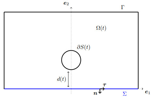
This paper is devoted to the mathematical analysis of the contact capabilities of the fluid-structure interaction (FSI) model with seepage reported in [Comput. Methods Appl. Mech., 392:114637, 2022]. In the case of a rigid disk moving over a fixed horizontal plane, we show that this model encompasses contact and hence removes the non collision paradox of traditional FSI models which rely on Dirichlet or Dirichlet/Navier boundary conditions. Numerical evidence on the theoretical results is also provided.

| [1] |
C. Ager, B. Schott, A. Vuong, A. Popp, W. A. Wall, A consistent approach for fluid-structure-contact interaction based on a porous flow model for rough surface contact, Int. J. Numer. Methods Eng., 119 (2019), 1345–1378. https://doi.org/10.1002/nme.6094 doi: 10.1002/nme.6094

|
| [2] | M. B. Allen, The mathematics of fluid flow through porous media, John Wiley & Sons, 2021. https://doi.org/10.1002/9781119663881 |
| [3] |
G. S. Beavers, D. D. Joseph, Boundary conditions at a naturally permeable wall, J. Fluid Mech., 30 (1967), 197–207. https://doi.org/10.1017/S0022112067001375 doi: 10.1017/S0022112067001375
|
| [4] |
M. Bercovier, Perturbation of mixed variational problems. Application to mixed finite element methods, RAIRO. Anal. Numér., 12 (1978), 211–236. https://doi.org/10.1051/m2an/1978120302111 doi: 10.1051/m2an/1978120302111
|
| [5] | M. Bogovskii, Solution of the first boundary value problem for an equation of continuity of an incompressible medium, Soviet Math. Dokl., 20 (1979), 1094–1098. |
| [6] | F. Boyer, P. Fabrie, Mathematical tools for the study of the incompressible Navier-Stokes equations and related models, Vol. 183, Springer Science & Business Media, 2012. |
| [7] |
E. Burman, M. A. Fernández, S. Frei, F. M. Gerosa, A mechanically consistent model for fluid-structure interactions with contact including seepage, Comput. Methods Appl. Mech. Eng., 392 (2022), 114637. https://doi.org/10.1016/j.cma.2022.114637 doi: 10.1016/j.cma.2022.114637
|
| [8] | C. Dobrzynski, P. Frey, Anisotropic delaunay mesh adaptation for unsteady simulations, In: R. V. Garimella, Proceedings of the 17th international Meshing Roundtable, Springer, 2008,177–194. https://doi.org/10.1007/978-3-540-87921-3_11 |
| [9] |
Q. Du, M. D. Gunzburger, L. S. Hou, J. Lee, Analysis of a linear fluid-structure interaction problem, Discrete Cont. Dyn. Syst., 9 (2003), 633–650. https://doi.org/10.3934/dcds.2003.9.633 doi: 10.3934/dcds.2003.9.633
|
| [10] | A. Ern, J. L. Guermond, Theory and practice of finite elements, Vol. 159, Springer, 2004. https://doi.org/10.1007/978-1-4757-4355-5 |
| [11] |
D. Gérard-Varet, M. Hillairet, Regularity issues in the problem of fluid structure interaction, Arch. Rational Mech. Anal., 195 (2010), 375–407. https://doi.org/10.1007/s00205-008-0202-9 doi: 10.1007/s00205-008-0202-9
|
| [12] |
D. Gérard-Varet, M. Hillairet, Computation of the drag force on a sphere close to a wall: the roughness issue, ESAIM: Math. Modell. Numer. Anal., 46 (2012), 1201–1224. https://doi.org/10.1051/m2an/2012001 doi: 10.1051/m2an/2012001
|
| [13] |
D. Gérard-Varet, M. Hillairet, C. Wang, The influence of boundary conditions on the contact problem in a 3D Navier-Stokes flow, J. Math. Pures Appl., 103 (2015), 1–38. https://doi.org/10.1016/j.matpur.2014.03.005 doi: 10.1016/j.matpur.2014.03.005
|
| [14] | V. Girault, P. A. Raviart, Finite element approximation of the Navier-Stokes equations, Vol. 749, Springer Berlin, 1979. https://doi.org/10.1007/BFb0063447 |
| [15] |
D. Gérard-Varet, M. Hillairet, Existence of weak solutions up to collision for viscous fluid-solid systems with slip, Commun. Pure Appl. Math., 67 (2014), 2022–2075. https://doi.org/10.1002/cpa.21523 doi: 10.1002/cpa.21523
|
| [16] | F. Hecht, New development in freefem++, J. Numer. Math., 20 (2012), 251–265. https://doi.org/10.1515/jnum-2012-0013 |
| [17] |
M. Hillairet, Lack of collision between solid bodies in a 2D incompressible viscous flow, Commun. Partial Differ. Eq., 32 (2007), 1345–1371. https://doi.org/10.1080/03605300601088740 doi: 10.1080/03605300601088740
|
| [18] |
M. Hillairet, A. Lozinski, M. Szopos, On discretization in time in simulations of particulate flows, Discrete Cont. Dyn. Syst.-Ser. B, 15 (2010), 935–956. https://doi.org/10.3934/dcdsb.2011.15.935 doi: 10.3934/dcdsb.2011.15.935
|
| [19] |
M. Hillairet, T. Takahashi, Collisions in three-dimensional fluid structure interaction problems, SIAM J. Math. Anal., 40 (2009), 2451–2477. https://doi.org/10.1137/080716074 doi: 10.1137/080716074
|
| [20] |
M. Hillairet, T. Takahashi, Existence of contacts for the motion of a rigid body into a viscous incompressible fluid with the tresca boundary conditions, Tunis. J. Math., 3 (2021), 447–468. https://doi.org/10.2140/tunis.2021.3.447 doi: 10.2140/tunis.2021.3.447
|
| [21] |
M. Hillairet, T. Takahashi, Blow up and grazing collision in viscous fluid solid interaction systems, Ann. Inst. Henri Poincaré C, Anal. non linéaire, 27 (2010), 291–313. https://doi.org/10.1016/j.anihpc.2009.09.007 doi: 10.1016/j.anihpc.2009.09.007
|
| [22] |
D. Kamensky, F. Xu, C. H. Lee, J. Yan, Y. Bazilevs, M. C. Hsu, A contact formulation based on a volumetric potential: application to isogeometric simulations of atrioventricular valves, Comput. Methods Appl. Mech. Eng., 330 (2018), 522–546. https://doi.org/10.1016/j.cma.2017.11.007 doi: 10.1016/j.cma.2017.11.007
|
| [23] |
N. Khaledian, P. F. Villard, M. O. Berger, Capturing contact in mitral valve dynamic closure with fluid-structure interaction simulation, Int. J. Comput. Assisted Radiol. Surg., 17 (2022), 1391–1398. https://doi.org/10.1007/s11548-022-02674-4 doi: 10.1007/s11548-022-02674-4
|
| [24] | J. L. Lions, E. Magenes, Non-homogeneous boundary value problems and applications: Vol. 1, Vol. 181, Springer Science & Business Media, 2012. https://doi.org/10.1007/978-3-642-65161-8 |
| [25] |
V. Martin, J. Jaffré, J. E. Roberts, Modeling fractures and barriers as interfaces for flow in porous media, SIAM J. Sci. Comput., 26 (2005), 1667–1691. https://doi.org/10.1137/S1064827503429363 doi: 10.1137/S1064827503429363
|
| [26] |
A. Mikelic, W. Jäger, On the interface boundary condition of Beavers, Joseph, and Saffman, SIAM J. Appl. Math., 60 (2000), 1111–1127. https://doi.org/10.1137/S003613999833678X doi: 10.1137/S003613999833678X
|
| [27] |
P. G. Saffman, On the boundary condition at the surface of a porous medium, Stud. Appl. Math., 50 (1971), 93–101. https://doi.org/10.1002/sapm197150293 doi: 10.1002/sapm197150293
|
| [28] | L. Tartar, The Lions-Magenes space $H_{00}^{1/2}(\Omega)$, In: An introduction to Sobolev spaces and interpolation Spaces, Lecture Notes of the Unione Matematica Italiana, Springer, 3 (2007), 159–161. https://doi.org/10.1007/978-3-540-71483-5_33 |
| [29] |
C. Wang, Strong solutions for the fluid-solid systems in a 2-D domain, Asymptotic Anal., 89 (2014), 263–306. https://doi.org/10.3233/ASY-141230 doi: 10.3233/ASY-141230
|


Figures(15) / Tables(1)

Marguerite Champion, Miguel A. Fernández, Céline Grandmont, Fabien Vergnet, Marina Vidrascu. On the analysis of a mechanically consistent model of fluid-structure-contact interaction[J]. Mathematics in Engineering, 2024, 6(3): 425-467. doi: 10.3934/mine.2024018


 DownLoad: