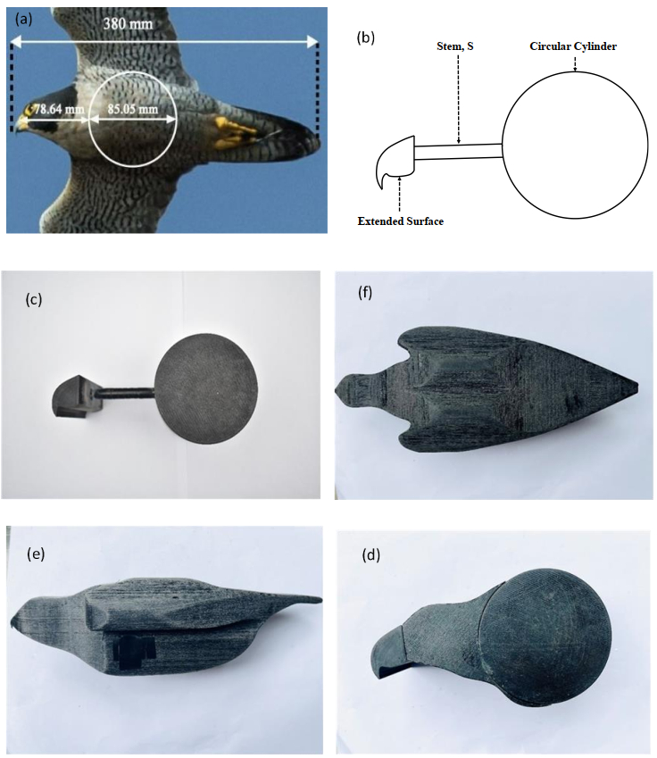
In the current work, the passive drag reduction of a circular cylinder for the subcritical Reynolds number range of 5.67×10⁴ to 1.79×10⁵ was computationally and experimentally investigated. First, inspired by nature, the aerodynamic drag coefficient of a whole Peregrine Falcon was measured in a subsonic wind tunnel for various angles of attack and Reynolds numbers (Re) and compared with the bare cylinder. At a 20° angle of attack and Re = 5.67×10⁴, the whole falcon model had a 75% lower drag coefficient than the bare cylinder. Later, with the moderate Falcon model, in which the falcon's beak and neck were linked to the cylinder as an extended surface, the drag coefficient decreased up to 72% in the subcritical Reynolds number zone. Finally, the extended surface with a falcon beak profile was connected to the cylinder with a stem and investigated both numerically and experimentally for various stem lengths, angles of attack, and Reynolds numbers. It was found that at low Re, the drag coefficient can be reduced by up to 47% for the stem length of 80 mm (L/D = 1.20) with an angle of attack 10°. The computational investigation yielded precise flow characteristics, and it was discovered that the stem length and the Re had a substantial influence on vortex generation and turbulent kinetic energy between the beak and cylinder, as well as downstream of the cylinder. Investigation revealed that percentile drag reduction was much lower for the whole Falcon model over a wide range of Reynolds numbers and positive angles of attack, which exist in nature. Similarly, when compared to the other stem lengths, the 60 mm stem length (L/D = 0.97) produced similar results to the whole Falcon model. The numerical results were well validated with the experimental results.
Citation: Shorob Alam Bhuiyan, Ikram Hossain, Redwan Hossain, Md. Sakib Ibn Mobarak Abir, Dewan Hasan Ahmed. Effect of a bioinspired upstream extended surface profile on flow characteristics and a drag coefficient of a circular cylinder[J]. Metascience in Aerospace, 2024, 1(2): 130-158. doi: 10.3934/mina.2024006
In the current work, the passive drag reduction of a circular cylinder for the subcritical Reynolds number range of 5.67×10⁴ to 1.79×10⁵ was computationally and experimentally investigated. First, inspired by nature, the aerodynamic drag coefficient of a whole Peregrine Falcon was measured in a subsonic wind tunnel for various angles of attack and Reynolds numbers (Re) and compared with the bare cylinder. At a 20° angle of attack and Re = 5.67×10⁴, the whole falcon model had a 75% lower drag coefficient than the bare cylinder. Later, with the moderate Falcon model, in which the falcon's beak and neck were linked to the cylinder as an extended surface, the drag coefficient decreased up to 72% in the subcritical Reynolds number zone. Finally, the extended surface with a falcon beak profile was connected to the cylinder with a stem and investigated both numerically and experimentally for various stem lengths, angles of attack, and Reynolds numbers. It was found that at low Re, the drag coefficient can be reduced by up to 47% for the stem length of 80 mm (L/D = 1.20) with an angle of attack 10°. The computational investigation yielded precise flow characteristics, and it was discovered that the stem length and the Re had a substantial influence on vortex generation and turbulent kinetic energy between the beak and cylinder, as well as downstream of the cylinder. Investigation revealed that percentile drag reduction was much lower for the whole Falcon model over a wide range of Reynolds numbers and positive angles of attack, which exist in nature. Similarly, when compared to the other stem lengths, the 60 mm stem length (L/D = 0.97) produced similar results to the whole Falcon model. The numerical results were well validated with the experimental results.

| [1] |
Sowoud KM, Al-Filfily AA, Abed BH (2020) Numerical Investigation of 2D Turbulent Flow past a Circular Cylinder at Lower Subcritical Reynolds Number. IOP Conf Ser Mater Sci Eng 881: 012160. https://doi.org/10.1088/1757-899X/881/1/012160 doi: 10.1088/1757-899X/881/1/012160

|
| [2] | Schlichting H, Gersten K (2016) Boundary-Layer Theory. Springer 1–799. |
| [3] |
Eun LC, Rafie ASM, Wiriadidjaja S, et al. (2018) An overview of passive and active drag reduction methods for bluff body of road vehicles. Int J Eng Technol 7: 53–56. https://doi.org/10.14419/ijet.v7i4.13.21328 doi: 10.14419/ijet.v7i4.13.21328
|
| [4] |
Frolov VA, Kozlova AS (2018) Influence of flat plate in front of circular cylinder on drag. AIP Conf Proc 2027: 1–9. https://doi.org/10.1063/1.5065182 doi: 10.1063/1.5065182
|
| [5] |
García-Baena C, Jiménez-González JI, Martínez-Bazán C (2021) Drag reduction of a blunt body through reconfiguration of rear flexible plates. Phys Fluids 33: 1–14. https://doi.org/10.1063/5.0046437 doi: 10.1063/5.0046437
|
| [6] |
Igarashi T (1981) Characteristics of the Flow around Two Circular Cylinders Arranged in Tandem : 1st Report. Bull JSME 24: 323–331. https://doi.org/10.1299/jsme1958.24.323 doi: 10.1299/jsme1958.24.323
|
| [7] |
Zdravkovich MM (1990) Conceptual overview of laminar and turbulent flows past smooth and rough circular cylinders. J Wind Eng Ind Aerodyn 33: 53–62. https://doi.org/10.1016/0167-6105(90)90020-D doi: 10.1016/0167-6105(90)90020-D
|
| [8] |
Xu G, Zhou Y (2004) Strouhal numbers in the wake of two inline cylinders. Exp Fluids 37: 248–56. https://doi.org/10.1007/s00348-004-0808-0 doi: 10.1007/s00348-004-0808-0
|
| [9] |
Wu J, Welch LW, Welsh MC, et al. (1994) Spanwise wake structures of a circular cylinder and two circular cylinders in tandem. Exp Therm Fluid Sci 9: 299–308. https://doi.org/10.1016/0894-1777(94)90032-9 doi: 10.1016/0894-1777(94)90032-9
|
| [10] |
Lin JC, Yang Y, Rockwell D (2002) Flow past two cylinders in tandem: instantaneous and averaged flow structure. J Fluids Struct 16: 1059–71. https://doi.org/10.1006/jfls.2002.0469 doi: 10.1006/jfls.2002.0469
|
| [11] |
Carmo BS, Meneghini JR, Sherwin SJ (2010) Secondary instabilities in the flow around two circular cylinders in tandem. J Fluid Mech 644: 395–431. https://doi.org/10.1017/S0022112009992473 doi: 10.1017/S0022112009992473
|
| [12] |
Lesage F, Gartshore IS (1987) A method of reducing drag and fluctuating side force on bluff bodies. J Wind Eng Ind Aerodyn 25: 229–45. https://doi.org/10.1016/0167-6105(87)90019-5 doi: 10.1016/0167-6105(87)90019-5
|
| [13] |
Alam MM, Zhou Y (2008) Strouhal numbers, forces and flow structures around two tandem cylinders of different diameters. J Fluids Struct 24: 505–26. https://doi.org/10.1016/j.jfluidstructs.2007.10.001 doi: 10.1016/j.jfluidstructs.2007.10.001
|
| [14] |
Zhao M, Cheng L, Teng B, et al. (2007) Hydrodynamic forces on dual cylinders of different diameters in steady currents. J Fluids Struct 23: 59–83. https://doi.org/10.1016/j.jfluidstructs.2006.07.003 doi: 10.1016/j.jfluidstructs.2006.07.003
|
| [15] |
Wang L, Alam MM, Zhou Y (2018) Two tandem cylinders of different diameters in cross-flow: effect of an upstream cylinder on wake dynamics. J Fluid Mech 836: 5–42. https://doi.org/10.1017/jfm.2017.735 doi: 10.1017/jfm.2017.735
|
| [16] |
Prasad A, Williamson CHK (1997) A method for the reduction of bluff body drag. J Wind Eng Ind Aerodyn 69-71: 155–167. https://doi.org/10.1016/S0167-6105(97)00151-7 doi: 10.1016/S0167-6105(97)00151-7
|
| [17] |
Han X, Wang J, Zhou B, et al. (2019) Numerical Simulation of Flow Control around a Circular Cylinder by Installing a Wedge-Shaped Device Upstream. J Mar Sci Eng 7: 422. https://doi.org/10.3390/jmse7120422 doi: 10.3390/jmse7120422
|
| [18] |
Law YZ, Jaiman RK (2017) Wake stabilization mechanism of low-drag suppression devices for vortex-induced vibration. J Fluids Struct 70: 428–449. https://doi.org/10.1016/j.jfluidstructs.2017.02.005 doi: 10.1016/j.jfluidstructs.2017.02.005
|
| [19] |
Alam MM, Sakamoto H, Zhou Y (2006) Effect of a T-shaped plate on reduction in fluid forces on two tandem cylinders in a cross-flow. J Wind Eng Ind Aerodyn 94: 525–551. https://doi.org/10.1016/j.jweia.2006.01.018 doi: 10.1016/j.jweia.2006.01.018
|
| [20] |
Bearman PW, Harvey JK (1993) Control of circular cylinder flow by the use of dimples. AIAA J 31: 1753–6. https://doi.org/10.2514/3.11844 doi: 10.2514/3.11844
|
| [21] |
Shih WCL, Wang C, Coles D, et al. (1993) Experiments on flow past rough circular cylinders at large Reynolds numbers. J Wind Eng Ind Aerodyn 49: 351–368. https://doi.org/10.1016/0167-6105(93)90030-R doi: 10.1016/0167-6105(93)90030-R
|
| [22] |
Yan F, Yang H, Wang L (2021) Study of the Drag Reduction Characteristics of Circular Cylinder with Dimpled Surface. Water 13: 197. https://doi.org/10.3390/w13020197 doi: 10.3390/w13020197
|
| [23] |
Yokoi Y, Igarashi T, Hirao K (2011) The Study about Drag Reduction of a Circular Cylinder with Grooves. J Fluid Sci Technol 6: 637–650. https://doi.org/10.1299/jfst.6.637 doi: 10.1299/jfst.6.637
|
| [24] |
Haque MA, Rauf MA, Ahmed DH (2017) Investigation of Drag Coefficient at Subcritical and Critical Reynolds Number Region for Circular Cylinder with Helical Grooves. Int J Marit Technol 8: 25–33. https://doi.org/10.29252/ijmt.8.25 doi: 10.29252/ijmt.8.25
|
| [25] | Haidary FM, Mazumder A, Hasan MR, et al. (2020) Investigation for the drag reduction by introducing a passage through a circular cylinder. Ann Eng 1: 1–13. |
| [26] |
Asif MA, Gupta AD, Rana MJ, et al. (2016) Investigation of drag reduction through a flapping mechanism on circular cylinder. AIP Conf Proc 1754: 1–5. https://doi.org/10.1063/1.4958374 doi: 10.1063/1.4958374
|
| [27] |
Gehrke A, Richeux J, Uksul E, et al. (2022) Aeroelastic characterisation of a bio-inspired flapping membrane wing. Bioinspir Biomim 17: 065004. https://doi.org/10.1088/1748-3190/ac8632 doi: 10.1088/1748-3190/ac8632
|
| [28] |
Buoso S, Dickinson BT, Palacios R (2017) Bat-inspired integrally actuated membrane wings with leading-edge sensing. Bioinspir Biomim 13: 016013. https://doi.org/10.1088/1748-3190/aa9a7b doi: 10.1088/1748-3190/aa9a7b
|
| [29] |
Shoshe MAMS, Islam A, Ahmed DH (2021) Effect of an upstream extended surface on reduction of total drag for finite cylinders in turbulent flow. Int J Fluid Mech Res 48: 27–44. https://doi.org/10.1615/InterJFluidMechRes.2021038255 doi: 10.1615/InterJFluidMechRes.2021038255
|
| [30] |
Islam A, Shoshe MAMS, Ahmed DH (2023) Reduction of Total Drag for Finite Cylinders in Turbulent Flow with a Half-C Shape Upstream Body. Int J Fluid Mech Res 50: 41–53. https://doi.org/10.1615/InterJFluidMechRes.2022045488 doi: 10.1615/InterJFluidMechRes.2022045488
|
| [31] |
Ghosh A, Gupta P, Jayant, et al. (2021) Metaheuristic optimization framework for drag reduction using bioinspired surface riblets. arXiv 2: 1–7. https://doi.org/10.48550/arXiv.2109.09650 doi: 10.48550/arXiv.2109.09650
|
| [32] |
Siddiqui NA, Agelin-Chaab M (2021) Nature-inspired solutions to bluff body aerodynamic problems: A review. J Mech Eng Sci 15: 1–52. https://doi.org/10.15282/jmes.15.2.2021.13.0638 doi: 10.15282/jmes.15.2.2021.13.0638
|
| [33] |
Cheney JA, Stevenson JPJ, Durston NE, et al. (2021) Raptor wing morphing with flight speed. J R Soc Interface 18: 1–14. https://doi.org/10.1098/rsif.2021.0349 doi: 10.1098/rsif.2021.0349
|
| [34] |
Sigrest P, Wu N, Inman DJ (2023) Energy considerations and flow fields over whiffling-inspired wings. Bioinspir Biomim 18: 046007. https://doi.org/10.1088/1748-3190/acd28f doi: 10.1088/1748-3190/acd28f
|
| [35] |
Bhardwaj H, Cai X, Win LST, et al. (2023) Nature-inspired in-flight foldable rotorcraft. Bioinspir Biomim 18: 46012. https://doi.org/10.1088/1748-3190/acd739 doi: 10.1088/1748-3190/acd739
|
| [36] |
Selim O, Gowree ER, Lagemann C, et al. (2021) Peregrine Falcon's Dive: Pullout Maneuver and Flight Control Through Wing Morphing. AIAA J 59: 3979–87. https://doi.org/10.2514/1.J060052 doi: 10.2514/1.J060052
|
| [37] |
Ponitz B, Schmitz A, Fischer D, et al. (2014) Diving-flight aerodynamics of a peregrine falcon (Falco peregrinus). PLoS One 9: e86506. https://doi.org/10.1371/journal.pone.0086506 doi: 10.1371/journal.pone.0086506
|
| [38] |
Pérez MG, Vakkilainen E (2019) A comparison of turbulence models and two and three dimensional meshes for unsteady CFD ash deposition tools. Fuel 237: 806–811. https://doi.org/10.1016/j.fuel.2018.10.066 doi: 10.1016/j.fuel.2018.10.066
|
| [39] |
Nazari S, Zamani M, Moshizi SA (2018) Comparison between two-dimensional and three-dimensional computational fluid dynamics techniques for two straight-bladed vertical-axis wind turbines in inline arrangement. Wind Eng 42: 47–64. https://doi.org/10.1177/0309524X18780384 doi: 10.1177/0309524X18780384
|
| [40] |
Stringer RM, Zang J, Hillis AJ (2014) Unsteady RANS computations of flow around a circular cylinder for a wide range of Reynolds numbers. Ocean Eng 87: 1–9. https://doi.org/10.1016/j.oceaneng.2014.04.017 doi: 10.1016/j.oceaneng.2014.04.017
|
| [41] |
Rafi AH, Haque MR, Ahmed DH (2022) Two-dimensional analogies to the deformation characteristics of a falling droplet and its collision. Archive Mech Eng 69: 21–43. https://doi.org/10.24425/ame.2021.139649 doi: 10.24425/ame.2021.139649
|
| [42] | Anderson JD (2011) Fundamentals of Aerodynamics (New York: McGraw-Hill Education). |
| [43] |
Johansson C, Linder ET, Hardin P, et al. (1998) Bill and body size in the peregrine falcon, north versus south: Is size adaptive? J Biogeogr 25: 265–273. https://doi.org/10.1046/j.1365-2699.1998.252191.x doi: 10.1046/j.1365-2699.1998.252191.x
|
| [44] | Holman JP (2011) Experimental Methods for Engineers (New York: McGraw-Hill), 60–165. |
| [45] |
Menter FR, Langtry RB, Likki SR, et al. (2006) A correlation-based transition model using local variables - Part Ⅰ: Model formulation. J Turbomach 128: 413–422. https://doi.org/10.1115/1.2184352 doi: 10.1115/1.2184352
|
| [46] | Malan P, Suluksna K, Juntasaro E (2009) Calibrating the γ-Reθ transition model for commercial CFD. 47th AIAA Aerospace Sciences Meeting including the New Horizons Forum and Aerospace Exposition (Orlando). https://doi.org/10.2514/6.2009-1142 |
| [47] | Menter FR (1993) Improved Two-Equation κ-ω Turbulence Models for Aerodynamic Flows. NASA TM 103975. https://doi.org/10.2514/6.1993-2906 |
| [48] | Munson BR, Young DF, Okiishi TH (1998) Fundamentals of fluid mechanics (Wiley). |
| [49] |
Rosetti GF, Vaz G, Fujarra ALC (2012) URANS calculations for smooth circular cylinder flow in a wide range of reynolds numbers: Solution verification and validation. J Fluids Eng Trans ASME 134: 121103. https://doi.org/10.1115/1.4007571 doi: 10.1115/1.4007571
|
| [50] |
Yuce MI, Kareem DA (2016) A numerical analysis of fluid flow around circular and square cylinders. J Am Water Works Assoc 108: 546–554. https://doi.org/10.5942/jawwa.2016.108.0141 doi: 10.5942/jawwa.2016.108.0141
|
| [51] | Hoener SF (1965) Pressure Drag Fluid Dynsmic Drag (New York, United States: Hoener Fluid Dynamics), 5–8. |
| [52] |
Achenbach E (1971) Influence of surface roughness on the cross-flow around a circular cylinder. J Fluid Mech 46: 321–335. https://doi.org/10.1017/S0022112071000569 doi: 10.1017/S0022112071000569
|
| [53] |
Hojo T (2015) Control of flow around a circular cylinder using a patterned surface. WIT Transactions on Modelling and Simulation 12: 245–256. https://doi.org/10.2495/CMEM150221 doi: 10.2495/CMEM150221
|
| [54] | Selig MS (2003) Low Reynolds Number Airfoil Design Lecture Notes, 1–43. |
| [55] |
Sohankar A, Khodadadi M, Rangraz E, et al. (2019) Control of flow and heat transfer over two inline square cylinders. Phys Fluids 31: 123604. https://doi.org/10.1063/1.5128751 doi: 10.1063/1.5128751
|
| [56] |
Aguedal L, Semmar D, Berrouk AS, et al. (2018) 3D vortex structure investigation using Large Eddy Simulation of flow around a rotary oscillating circular cylinder. Eur J Mech B/Fluids 71: 113–125. https://doi.org/10.1016/j.euromechflu.2018.04.001 doi: 10.1016/j.euromechflu.2018.04.001
|
| [57] | Ji L, Du H, Yang LJ, et al. (2023) Research on the drag reduction characteristics and mechanism of a cylinder covered with porous media. AIP Adv 13: 035220. https://doi.org/10.1063/5.0141832 |
| [58] |
Qi J, Qi Y, Chen Q, et al. (2022) A study of drag reduction on cylinders with different v-groove depths on the surface. Water 14: 36. https://doi.org/10.3390/w14010036 doi: 10.3390/w14010036
|


Figures(15) / Tables(1)
Shorob Alam Bhuiyan, Ikram Hossain, Redwan Hossain, Md. Sakib Ibn Mobarak Abir, Dewan Hasan Ahmed. Effect of a bioinspired upstream extended surface profile on flow characteristics and a drag coefficient of a circular cylinder[J]. Metascience in Aerospace, 2024, 1(2): 130-158. doi: 10.3934/mina.2024006


 DownLoad: