Current trends in the management of pilonidal sinus disease and its outcome in a periphery hospital

Fauwaz Fahad Alrashid; Saadeldin Ahmed Idris; Abdul Ghani Qureshi; Fauwaz Fahad Alrashid; Saadeldin Ahmed Idris; Abdul Ghani Qureshi

doi:10.3934/medsci.2021008

AIMS Medical Science

2021, Volume 8, Issue 1: 70-79. doi: 10.3934/medsci.2021008

Previous Article Next Article

Research article

Current trends in the management of pilonidal sinus disease and its outcome in a periphery hospital

1.
Department of Surgery, College of Medicine, University of Hail, KSA
2.
Department of Surgery, Almikhwah General Hospital, Al-Baha, KSA

Received: 08 December 2020 Accepted: 02 March 2021 Published: 09 March 2021

Background
The attention of surgeons to pilonidal sinus disease is increasing. We aimed to estimate the incidence of Pilonidal sinus disease, and verify the employed management and its outcome in term of surgical site infection, recurrence and patients' satisfaction.
Methods
A cohort study included 224 patients with pilonidal sinus disease (Jan 2014 to April 2020).
Results
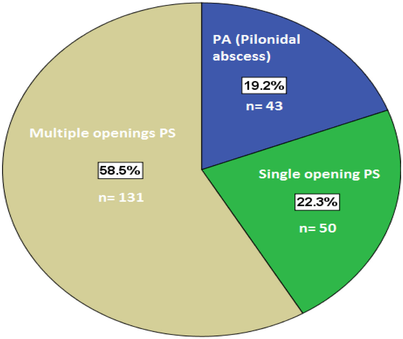
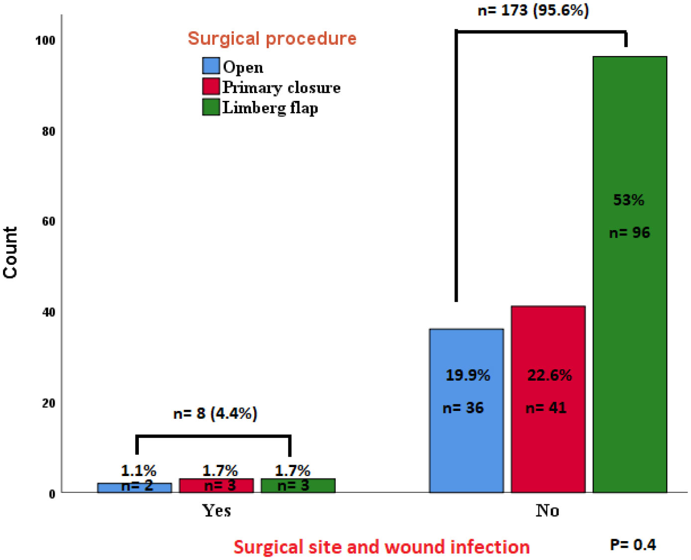
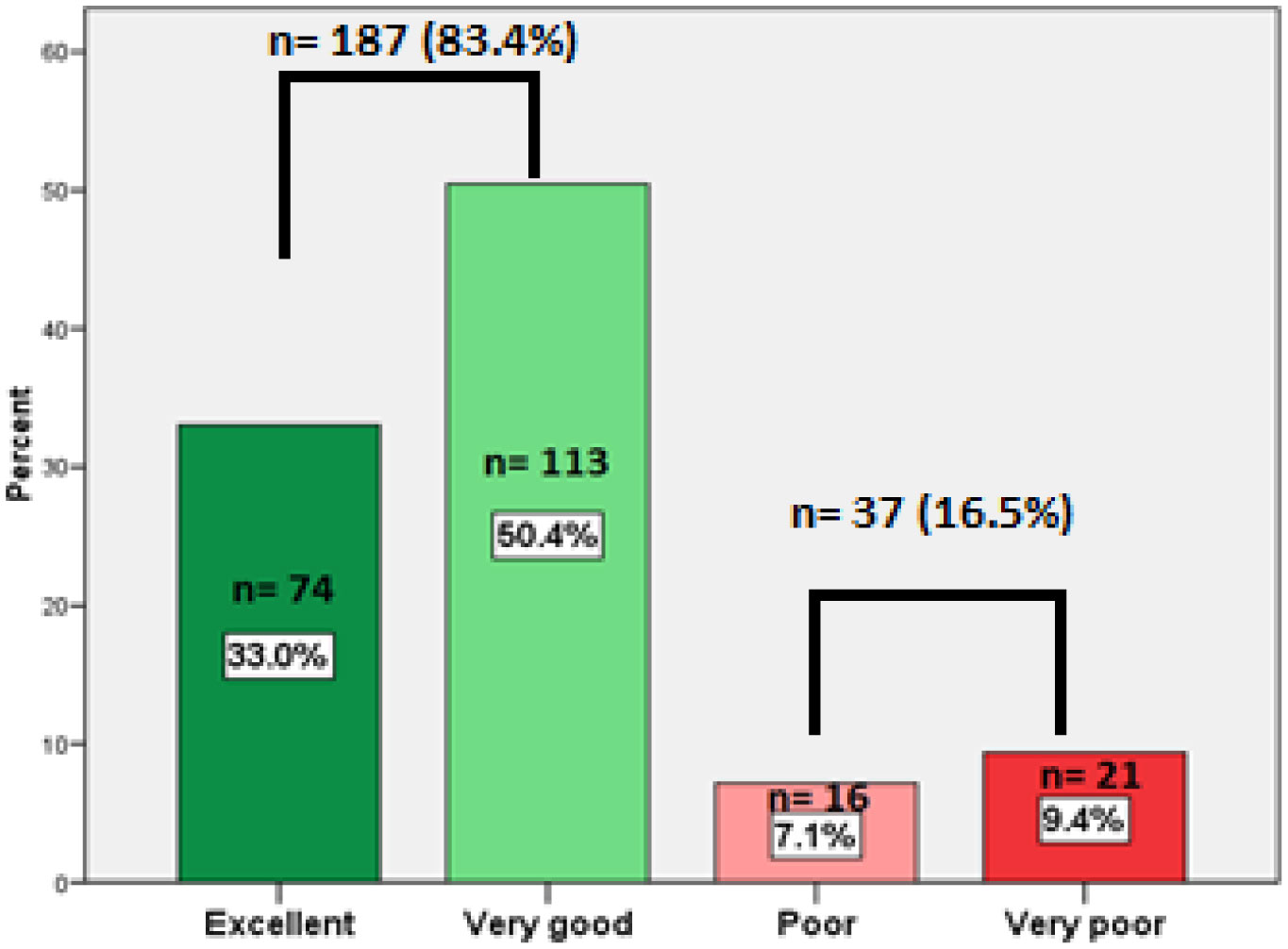
Mean age was 23.83 ± 4.9 years, with male predominance (male to female ratio of 2.25:1). Incidence of pilonidal sinus disease was 2.9% of all surgical clinic population. Mean duration of symptoms was 65.8 ± 50.7 days. Majority (80.8%) had chronic pilonidal sinus, whereas the remainder 19.2% had acute onset with abscess. In pilonidal sinus the surgical modality was fashioned according to the extent of the disease keeping in mind the number of sinus opening in form of Limberg flap (44.2%), primary closure (19.6%), or laid open to heal by secondary intention (17%). Recurrence of pilonidal sinus was seen in 2.2% and not affected by the procedure employed (P = 0.4). Whereas, in cases of pilonidal abscess the recurrence rate was 27.9%. The difference was significant (p = 0.00001). Over all patients' satisfaction was very good/excellent in 187 (83.4%).
Conclusions
To reduce congestion of the operating lists in central hospitals, one can use a clear criterion based on the extent of the disease and the number of sinus openings, this will facilitate the management of pilonidal sinus disease in peripheral hospital settings, and comparable results can be achieved in terms of recurrence rate and patient satisfaction.
- patients' satisfaction,
- pilonidal abscess,
- pilonidal disease,
- pilonidal sinus,
- surgery
Citation: Fauwaz Fahad Alrashid, Saadeldin Ahmed Idris, Abdul Ghani Qureshi. Current trends in the management of pilonidal sinus disease and its outcome in a periphery hospital[J]. AIMS Medical Science, 2021, 8(1): 70-79. doi: 10.3934/medsci.2021008

Related Papers:

Abstract

Background

The attention of surgeons to pilonidal sinus disease is increasing. We aimed to estimate the incidence of Pilonidal sinus disease, and verify the employed management and its outcome in term of surgical site infection, recurrence and patients' satisfaction.

Methods

A cohort study included 224 patients with pilonidal sinus disease (Jan 2014 to April 2020).

Results

Mean age was 23.83 ± 4.9 years, with male predominance (male to female ratio of 2.25:1). Incidence of pilonidal sinus disease was 2.9% of all surgical clinic population. Mean duration of symptoms was 65.8 ± 50.7 days. Majority (80.8%) had chronic pilonidal sinus, whereas the remainder 19.2% had acute onset with abscess. In pilonidal sinus the surgical modality was fashioned according to the extent of the disease keeping in mind the number of sinus opening in form of Limberg flap (44.2%), primary closure (19.6%), or laid open to heal by secondary intention (17%). Recurrence of pilonidal sinus was seen in 2.2% and not affected by the procedure employed (P = 0.4). Whereas, in cases of pilonidal abscess the recurrence rate was 27.9%. The difference was significant (p = 0.00001). Over all patients' satisfaction was very good/excellent in 187 (83.4%).

Conclusions

To reduce congestion of the operating lists in central hospitals, one can use a clear criterion based on the extent of the disease and the number of sinus openings, this will facilitate the management of pilonidal sinus disease in peripheral hospital settings, and comparable results can be achieved in terms of recurrence rate and patient satisfaction.

Abbreviations

Hidradenitis suppurativa

MGH

Almikhwah General Hospital

PSD

Pilonidal sinus disease

SSI

Surgical site infection

Pilonidal sinus

Pilonidal abscess

Acknowledgments

We are over helmed in all humbleness and gratefulness to acknowledge our depth to all those who have helped us to put these ideas, well above the level of simplicity and into something concrete. Special thanks to the employee in medical record department without their help this work couldn't see the light.

Conflict of interest

The authors declare that there is no conflict of interest regarding the publication of this article.

References

[1]	Lim J, Shabbir J (2019) Pilonidal sinus disease—a literature review. World J Surg Surgical Res 2: 1117.
[2]	Karandikar S, Naik NG (2017) Retrospective analysis of 30 cases of pilonidal sinus by various techniques of conservative and surgical management and review of literature. Int Surg J 4: 291-295. doi: 10.18203/2349-2902.isj20164457
[3]	Stauffer VK, Luedi MM, Kauf P, et al. (2018) Common surgical procedures in pilonidal sinus disease: a meta-analysis, merged data analysis, and comprehensive study on recurrence. Sci Rep 8: 1-28. doi: 10.1038/s41598-017-17765-5
[4]	Doll D, Orlik A, Maier K, et al. (2019) Impact of geography and surgical approach on recurrence in global pilonidal sinus disease. Sci Rep 9: 1-24. doi: 10.1038/s41598-019-51159-z
[5]	Darwish AA, Eskandaros MS, Hegab A (2017) Sacrococcygeal pilonidal sinus: modified sinotomy versus lay-open, limited excision, and primary closure. Egypt J Surg 36: 13-19. doi: 10.4103/1110-1121.199901
[6]	Mahmood F, Hussain A, Akingboye A (2020) Pilonidal sinus disease: review of current practice and prospects for endoscopic treatment. Ann Med Surg 57: 212-217. doi: 10.1016/j.amsu.2020.07.050
[7]	Lamdark T, Vuille-dit-Bille RN, Bielicki IN, et al. (2020) Treatment strategies for pilonidal sinus disease in Switzerland and Austria. Medicina 56: 341. doi: 10.3390/medicina56070341
[8]	Duman K, Gırgın M, Harlak A (2017) Prevalence of sacrococcygeal pilonidal disease in Turkey. Asian J Surg 40: 434-437. doi: 10.1016/j.asjsur.2016.04.001
[9]	Rao J, Deora H, Mandia R (2015) A retrospective study of 40 cases of pilonidal sinus with excision of tract and Z-plasty as treatment of choice for both primary and recurrent cases. Indian J Surg 77: 691-693. doi: 10.1007/s12262-013-0983-4
[10]	Mohamed Abd-Elfattah AM, Elsayed Fahmi KS, Eltih OA, et al. (2020) The Karydakis Flap Versus the Limberg Flap in the treatment of pilonidal sinus disease. Zagazig Univ Med J 26: 900-907.
[11]	Aysan E, Ilhan M, Bektas H, et al. (2013) Prevalence of sacrococcygeal pilonidal sinus as a silent disease. Surg Today 43: 1286-1289. doi: 10.1007/s00595-012-0433-0
[12]	Burnett D, Smith SR, Young CJ (2018) The surgical management of pilonidal disease is uncertain because of high recurrence rates. Cureus 10: e2625.
[13]	Bascom J (2008) Surgical treatment of pilonidal disease. BMJ 336: 842-843. doi: 10.1136/bmj.39535.397292.BE
[14]	Iesalnieks I, Ommer A, Petersen S, et al. (2016) German national guideline on the management of pilonidal disease. Langenbecks Arch Surg 401: 599-609. doi: 10.1007/s00423-016-1463-7
[15]	Brown SR, Lund JN (2019) The evidence base for pilonidal sinus surgery is the pits. Tech Coloproctol 23: 1173-1175. doi: 10.1007/s10151-019-02116-5
[16]	Søndenaa K, Nesvik I, Andersen E, et al. (1995) Bacteriology and complications of chronic pilonidal sinus treated with excision and primary suture. Int J Colorectal Dis 10: 161-166. doi: 10.1007/BF00298540
[17]	Chaudhuri A, Bekdash BA (2005) Single-dose metronidazole versus 5-day multidrug antibiotic regimen in excision of pilonidal sinuses with primary closure: a prospective randomized controlled double-blinded study. Int J Colorectal Dis 17: 355-358. doi: 10.1007/s00384-002-0416-5
[18]	Miocinović M, Horzić M, Bunoza D (2001) The prevalence of anaerobic infection in pilonidal sinus of the sacrococcygeal region and its effect on the complications. Acta Med Croatica 55: 87-90.
[19]	Awad MMS, Saad KM (2006) Does closure of chronic pilonidal sinus still remain a matter of debate after bilateral rotation flap? (N-shaped closure technique). Indian J Plast Surg 39: 157-162. doi: 10.4103/0970-0358.29545
[20]	Badr ML, Mohammed MA, Zahran SM (2018) Prospective randomized comparative study of a Karydakis flap versus ordinary midline closure for the treatment of primary pilonidal sinus. Menoufia Med J 31: 102-107.
[21]	Azab AS, Kamal MS, Saad RA, et al. (1984) Radical cure of pilonidal sinus by a transposition rhomboid flap. Br J Surg 71: 154-155. doi: 10.1002/bjs.1800710227
[22]	Mahdy T, Mahdy T, Gaertner WB, et al. (2008) Surgical treatment of the pilonidal disease: primary closure or flap reconstruction after excision. Dis Colon Rectum 51: 1816-1822. doi: 10.1007/s10350-008-9436-8
[23]	Akca T, Colak T, Ustunsoy B, et al. (2005) Randomized clinical trial comparing primary closure with the Limberg flap in the treatment of primary sacrococcygeal pilonidal disease. BMJ 92: 1081-1084.
[24]	Al-Khayat H, Al-Khayat H, Sadeq A, et al. (2007) Risk factors for wound complication in pilonidal sinus procedures. J Am Coll Surg 205: 439-444. doi: 10.1016/j.jamcollsurg.2007.04.034
[25]	Kanlioz M, Ekici U (2019) Complications during the recovery period after pilonidal sinus surgery. Cureus 11: e4501.
[26]	Iesalnieks I, Ommer A (2019) The management of pilonidal sinus. Dtsch Arztebl Int 116: 12-21.
[27]	Clothier PR, Haywood IR (1984) The natural history of the post anal (pilonidal) sinus. Ann R Coll Surg Engl 66: 201-203.
[28]	Mustafi N, Engels P (2016) Post-surgical wound management of pilonidal cysts with a haemoglobin spray: a case series. J Wound Care 25: 191-198. doi: 10.12968/jowc.2016.25.4.191
[29]	Kayaalp C, Olmez A, Aydin C, et al. (2010) Investigation of a one-time phenol application for pilonidal disease. Med Princ Pract 19: 212-215. doi: 10.1159/000285291

Reader Comments

your name:*

Email:*
© 2021 the Author(s), licensee AIMS Press. This is an open access article distributed under the terms of the Creative Commons Attribution License (http://creativecommons.org/licenses/by/4.0)