Loading [MathJax]/jax/element/mml/optable/BasicLatin.js
Review

Chitosan-Based Nanomaterials for Skin Regeneration

  • Chitosan (CS) is a renewable polysaccharide widely used for the preparation of biomaterials due to its special properties such as its biodegradability and biocompatibility, mucoadhesive behavior, and antibacterial and anti-inflammatory effects. These features are very important for biomedical applications, especially for tissue engineering and skin regeneration. From the clinical point of view, there is an increasing demand for the development of new materials/scaffolds with dual roles: the promotion of skin tissue repair and the simultaneous exertion of potent antimicrobial effects. Nanotechnology has been extensively employed in several pharmacological applications, including cutaneous tissue repair and antimicrobial treatments. The combination of CS and nanotechnology might create new avenues in tissue engineering. In this sense, this review presents and discusses recent advantages and challenges in the design of CS-based nanomaterials (in the form of nanofibers, composite nanoparticles, and nanogels) for cutaneous tissue regeneration. The combination of CS-based nanomaterials with other polymers, active drugs and metallic nanoparticles is also discussed from the viewpoint of designing suitable platforms for regenerative medicine and tissue engineering.

    Citation: Milena T. Pelegrino, Amedea B. Seabra. Chitosan-Based Nanomaterials for Skin Regeneration[J]. AIMS Medical Science, 2017, 4(3): 352-381. doi: 10.3934/medsci.2017.3.352

    Related Papers:

    [1] Qing Yang, Chuanzhi Bai, Dandan Yang . Finite-time stability of nonlinear stochastic ψ-Hilfer fractional systems with time delay. AIMS Mathematics, 2022, 7(10): 18837-18852. doi: 10.3934/math.20221037
    [2] Jingfeng Wang, Chuanzhi Bai . Finite-time stability of q-fractional damped difference systems with time delay. AIMS Mathematics, 2021, 6(11): 12011-12027. doi: 10.3934/math.2021696
    [3] Junsoo Lee, Wassim M. Haddad . On finite-time stability and stabilization of nonlinear hybrid dynamical systems. AIMS Mathematics, 2021, 6(6): 5535-5562. doi: 10.3934/math.2021328
    [4] Zhengqi Zhang, Huaiqin Wu . Cluster synchronization in finite/fixed time for semi-Markovian switching T-S fuzzy complex dynamical networks with discontinuous dynamic nodes. AIMS Mathematics, 2022, 7(7): 11942-11971. doi: 10.3934/math.2022666
    [5] Yanli Ma, Hamza Khalil, Akbar Zada, Ioan-Lucian Popa . Existence theory and stability analysis of neutral ψ–Hilfer fractional stochastic differential system with fractional noises and non-instantaneous impulses. AIMS Mathematics, 2024, 9(4): 8148-8173. doi: 10.3934/math.2024396
    [6] Tiecheng Zhang, Liyan Wang, Yuan Zhang, Jiangtao Deng . Finite-time stability for fractional-order fuzzy neural network with mixed delays and inertial terms. AIMS Mathematics, 2024, 9(7): 19176-19194. doi: 10.3934/math.2024935
    [7] Prabakaran Raghavendran, Tharmalingam Gunasekar, Irshad Ayoob, Nabil Mlaiki . AI-driven controllability analysis of fractional impulsive neutral Volterra-Fredholm integro-differential equations with state-dependent delay. AIMS Mathematics, 2025, 10(4): 9342-9368. doi: 10.3934/math.2025432
    [8] Yong-Ki Ma, Marimuthu Mohan Raja, Kottakkaran Sooppy Nisar, Anurag Shukla, Velusamy Vijayakumar . Results on controllability for Sobolev type fractional differential equations of order 1<r<2 with finite delay. AIMS Mathematics, 2022, 7(6): 10215-10233. doi: 10.3934/math.2022568
    [9] Jun Liu, Wenjing Deng, Shuqin Sun, Kaibo Shi . Novel fixed-time synchronization results of fractional-order fuzzy cellular neural networks with delays and interactions. AIMS Mathematics, 2024, 9(5): 13245-13264. doi: 10.3934/math.2024646
    [10] Yidan Wang, Li Xiao, Yanfeng Guo . Finite-time stability of singular switched systems with a time-varying delay based on an event-triggered mechanism. AIMS Mathematics, 2023, 8(1): 1901-1924. doi: 10.3934/math.2023098
  • Chitosan (CS) is a renewable polysaccharide widely used for the preparation of biomaterials due to its special properties such as its biodegradability and biocompatibility, mucoadhesive behavior, and antibacterial and anti-inflammatory effects. These features are very important for biomedical applications, especially for tissue engineering and skin regeneration. From the clinical point of view, there is an increasing demand for the development of new materials/scaffolds with dual roles: the promotion of skin tissue repair and the simultaneous exertion of potent antimicrobial effects. Nanotechnology has been extensively employed in several pharmacological applications, including cutaneous tissue repair and antimicrobial treatments. The combination of CS and nanotechnology might create new avenues in tissue engineering. In this sense, this review presents and discusses recent advantages and challenges in the design of CS-based nanomaterials (in the form of nanofibers, composite nanoparticles, and nanogels) for cutaneous tissue regeneration. The combination of CS-based nanomaterials with other polymers, active drugs and metallic nanoparticles is also discussed from the viewpoint of designing suitable platforms for regenerative medicine and tissue engineering.


    The interconnection between the dynamical behavior of discrete and continuous systems is referred to as a hybrid class. The concept of hybrid systems can be utilized to study the discrete dynamics of a model whenever the continuous form of the system has a suppressed effect. In networking, hybrid systems maximize the impact of new technology by integrating newly developed techniques with existing ones, thereby enhancing the efficiency of the constructed model. This type of system has gained remarkable attention in various evolving fields, such as networking and communications, industries, and circuit models [1,2,3]. The study of continuous-time models with switches at discrete time instants is referred to as switched systems. By abstracting away the discrete behavior and focusing on the possible switching patterns within a class, it is possible to derive switched systems from hybrid models. In the control design of systems with sub-modules, the switching mechanism plays a crucial role. This mechanism is categorized based on two criteria: time-dependent and state-dependent switches. In the case of switches which are dependent on the state, the space Rn is divided into a set of operating regions by a family of switching sequence. Now each of these regions is interlinked with a sub-module which is continuous. When the trajectory of the system cuts through switching surface, the state response of the system suddenly undergoes a change and jumps to a new region by means of a reset map, whereas, if we consider a switching sequence which is time dependent the system consists of a piecewise constant switching signal δ:[0,]P, where P is a finite positive set of integers. The discontinuities of a function δ at finite time instant is called switching time signals. Here, δ defines the active subsystem at each time instant. Existence of solution and its uniqueness for the uncertain class of the switched fractional model was presented in [4]. Positive solutions of switching models was established by [5]. Switching topologies of the multi-agent model was analyzed in [6].

    The examination of system behavior in the presence of time delay is a crucial aspect while designing physiological and circuit systems. Moreover, analyzation of delay effect has gained even more attention while designing control models. Significant study time-delay control models can be found in [7,8,9]. Controllability is one of the most important and effective aspects of studying and manipulating the designed model according to specific requirements. This approach helps refine differential models. The impact of impulses on a system plays a vital role in designing the control input, as it requires formulating a piecewise control input for each interval. Few methods to study the impulsive control systems and their stability are found in [10,11,12,13]. When it comes to nonlinear controllability, the two vital techniques used are fixed point and differential geometry [14,15,16,17]. Switched system combined with impulsive effects is more efficient to model the discontinuous dynamics. Existing literature provides a great range of solution methods for hybrid systems. [18] et al. discussed the controllability of switch perturbed system with delays. The geometric method to analyze the reachability of the switched linear system was presented in [19]. Controllability of multi-delay switched models was presented in [20]. Some recent results on relative cotrollability of fractional order systems can be found in [21,22]. There are very few works pertaining to the analysis on stability and controllability of the switched fractional system. To mention a few, T. Kaczorek in [23] established the asymptotic behavior of the linear switched positive fractional system. Stability of impulsive switched fractional conformable system was discussed in [24]. Boundedness and stability of switched fractional models over finite time period was discussed in [25]. In [26], the authors discussed the controllability criteria for the Hilfer switched dynamical model. Relative controllability of the switched nonlinear fractional order system was established in [16]. Study on the control results of the nonlocal switching system can be found in [27]. Finite-time stability (FTS) refers to the study of whether a system's state remains within a predefined threshold over a fixed time interval. In other words, FTS ensures that the system's solution does not exceed a certain bound within a given time horizon, regardless of external disturbances or initial conditions. Unlike traditional asymptotic stability, which focuses on long-term behavior, FTS is particularly useful in scenarios where maintaining system constraints over a finite duration is critical, such as in control applications, robotics, and networked systems.

    One of the key criteria for achieving FTS is ensuring that the system variables remain bounded within the specified time frame. This boundedness is essential in many real-world applications where transient behavior plays a crucial role, such as in aerospace systems, power grids, and biological models. Various techniques, including Lyapunov-based methods, comparison principles, and differential inequalities, are commonly employed to establish sufficient conditions for finite-time stability.

    Due to its significance in practical applications, FTS has been a subject of extensive research in recent years. Numerous studies explore different approaches to analyze and enhance FTS, particularly in hybrid and switched systems, where impulsive effects and delays introduce additional complexities. Researchers continue to develop novel methodologies and theoretical frameworks to improve stability guarantees in such systems, making FTS an active and evolving area of study in control theory and applied mathematics. Work presented in [28] analyzes the FTS of neutral fractional system in-terms of fixed point results. Thresholds for impulsive singular systems to admit FTS was studied in [29]. Switching system stability was examined in [15,30]. A lot of informative results on FTS and how essentially it affects the analyzation of differential models are discussed in [2,14,28,29,31,32,33,34]. Comparative studies on stability and controllability of switching systems for various derivatives of fractional order are presented in [15,26,35,36,37,38,39].

    A careful examination of the aforementioned research works reveals that the general form of the solution is not easily deduced when the switched system is subject to time delays that occur at different time instants, particularly when coupled with nonlinear perturbations. This complexity presents a significant challenge in the analysis and control of such systems. In this context, this work investigates the finite-time stability and relative-type control criteria for fractional-order switched impulsive systems with delays occurring at distinct time instants. The aim is to develop effective control strategies that account for the interplay between time delays, nonlinearity, and fractional dynamics.

    (cDγy)(τ)=Hδ(τ)y(τd)+Pδ(τ)w(τρ)+Qδ(τ)(τ,y(τ),τ0g(τ,η,y(η))dη),τ(τl1,τl],Δy(τ)=Eδ(τ)y(τ),τ=τl,y(τ)=ζ1(τ),τ0dττ0,ζ1(τ)C([τ0d,τ0],Rn),w(τ)=ζ2(τ),τ0ρττ0,ζ2(τ)C([τ0ρ,τ0],Rm), (1.1)

    where the derivative order is γ(12,1), the state response vector is y(τ)Rn, and w(τ)Rm. Then, d>0,ρ>0 represents the time delay in the state and control input. δ(τ):[0,]SK1=1,...,K represents the switching function which is left continuous. At the instant δ(τ)=j the jth subsystem (Hj,Pj,Qj) will be active. Jump at the instant τl is denoted by Δy(τl)+y(τl)=y(τ+l). The matrices are HjRn×n,PjRn×m and QjC([τ0,τl]×Rn×Rn,Rn).Eδ(τ):RnRn, represents the impulsive function. Let rl=τlτl1 represent the dwell time. At this point, it is important to note the switching signals and perturbations occur simultaneously and, therefore synchronize at τl. As a first step, we begin by deducing the solution of system (1.1) to analyze the stability and control results. Consider the following system

    (cDγy)(τ)=Hy(τd)+Q(τ),ττ0,y(τ)=ζ1(τ),τ0dττ0,ζ1(τ)C([τ0d,τ0],Rn). (1.2)

    The authors in [40] proposed the solution of (1.2) as

    ˜y(τ)=ZH(ττ0)γdζ1(τd)+τ0τ0dZH(τdν)γdζ1(ν)dν+ττ0ZH(τν)γd,γQ(ν)dν, (1.3)

    where ZH.γd and ZH.γd,γ will be described later. It is more complicated to evaluate the solution of (1.1) as in the form of (1.3); hence, we first establish improvised form of (1.3) to deduce the state response of (1.1).

    While there is significant research on linear models and stability criteria for fractional-order differential equations, the nonlinear analytical methods specific to FTS systems remain less explored. Furthermore, there is a lack of generalization in the thresholds for FTS across different models. The study of generalized models and their identifiability or invertibility in the context of fractional delays has not been thoroughly established in previous works, especially concerning systems with nonlinear dynamics. The paper addresses identifiability and invertibility of generalized fractional models, which is not commonly explored in the literature. This contributes to the practical application of these models, particularly in fields involving parameter estimation and system identification. This integrated approach offers a more robust validation of the theoretical findings, providing a clear pathway from mathematical derivations to practical implementation. This was largely missing from earlier research where either theoretical or numerical methods were treated separately. We try to propose a piecewise continuous solution in the form of the delayed matrix Mittag Leffler function. Then, we deduce the require bound for (1.1) to admit finite time period stability. Further, analytical and fixed point techniques will be used to analyze the relative control results of (1.1). The framework of the article is outlined as follows:

    In Section 2, we discuss the basic results, integral inequalities, and definitions which are required for theoretical study. The thresholds required for FTS are deduced in Section 3. In Section 4, we provide a nonlinear analytical study using theorems, such as the fixed point for (1.1), to be relatively controllable. In Section 5, we substantiate our study with concrete numerical simulations.

    Let us take into account the vector space Rn with H=λmax(HTH) as the matrix norm, where λmax(H) is the largest eigenvalue of the matrix H. Then, J=P.C.([τ0d,τN],Rn) denoted the piecewise continuous Banach space function. Let y=sup Moreover, let \| \mathcal{y} \|_{L^{2}[\mathtt{τ}_{0}, \mathtt{τ}_{N}]} = \big(\int_{\mathtt{τ}_{0}}^{\mathtt{τ}_{N}} \| \mathcal{y}(\mathtt{ν}) \|^{2}d\mathtt{ν}\big)^{\frac{1}{2}} be the square functions which are integrable. The important assumption that we need to consider is r_{l} > \max\{d, \mathtt{ρ}\}.

    Definition 2.1. [16] Let \{\mathtt{τ}_{l}\}_{1}^{N} be a sequence of time periods. Then, \mathtt{δ}:[\mathtt{τ}_{0}, \mathtt{τ}_{N}]\rightarrow \mathcal{S}_{1}^{K} is defined as an admissible switch if \mathtt{δ}(\mathtt{τ}) = \mathtt{δ}(\mathtt{τ}_{l}^{+}) = \mathtt{δ}(\mathtt{τ}_{l+1}), \mathtt{τ} \in(\mathtt{τ}_{l-1}, \mathtt{τ}_{l}] , and \mathtt{δ}(\mathtt{τ}_{0}) = \mathtt{δ}(\mathtt{τ}_{0}^{+}) .

    Definition 2.2. [16] For any given initial functions \mathtt{ζ}_{1}(\mathtt{τ}) and \mathtt{ζ}_{2}(\mathtt{τ}) , the relative type controllability of (1.1) with respect to the \{\mathtt{τ}_{l}\}_{l = 1}^{N} is guaranteed if for the admissible signal \mathtt{δ}(\mathtt{τ}) and the input \mathcal{w}\in \mathcal{L}^{2}([\mathtt{τ}_{0}, \mathtt{τ}_{N}-\mathtt{ρ}], \mathfrak{R}^{m}) in such a way that \mathcal{y}(\mathtt{τ}_{N}) = \mathcal{y}_{f}.

    Definition 2.3. [7] The differential operator in the sense of Riemann-Liouville with order \mathtt{γ}\in(0, 1) of a function \mathcal{y}:[0, \infty)\rightarrow \mathfrak{R} is given as (^{RL} {D}^{\mathtt{γ}} \mathcal{y})(\mathtt{τ}) = \dfrac{1}{\Gamma(1-\mathtt{γ})}\dfrac{d}{d\, \mathtt{τ}}\int_{0}^{\mathtt{τ}} \dfrac{\mathcal{y}(\mathtt{ν})}{(\mathtt{τ}-\mathtt{ν})^\mathtt{γ}} d\mathtt{ν}.

    Definition 2.4. [30] The differential operator in the sense of Caputo with order \mathtt{γ}\in(0, 1) of a function \mathcal{y}:[0, \infty)\rightarrow \mathfrak{R} is given as (^{C} {D}^{\mathtt{γ}} \mathcal{y})(\mathtt{τ}) = (^{RL} {D}^{\mathtt{γ}} \mathcal{y})(\mathtt{τ})-\dfrac{\mathcal{y}(0)}{\Gamma(1-\mathtt{γ})}\mathtt{τ}^{-\mathtt{γ}}.

    Definition 2.5. [7] The Mittag-Leffler (ML) functions \mathcal{E}_{\mathtt{γ}} and \mathcal{E}_{\mathtt{γ}, \mathtt{ν}} are given as

    \begin{align*} \mathcal{E}_{\mathtt{γ}}(\mathtt{τ})& = \sum_{l = 0}^{\infty} \dfrac{\mathtt{τ}^{l}}{\Gamma(l\mathtt{γ}+1)}, \mathtt{γ} > 0,\\ \mathcal{E}_{\mathtt{γ},\mathtt{ν}}(\mathtt{τ})& = \sum_{l = 0}^{\infty} \dfrac{\mathtt{τ}^{l}}{\Gamma(l\mathtt{γ}+\mathtt{ν})}, (\mathtt{γ}, \mathtt{ν}) > 0. \end{align*}

    Moreover, we have the integral identity

    \begin{align*} \int_{\mathcal{a}}^{\mathcal{b}} (\mathtt{τ}-\mathtt{ν})^{\mathtt{γ}-1}\mathcal{E}_{\mathtt{γ},\mathtt{γ}}(\mathtt{λ}(\mathtt{τ}-\mathtt{ν})^{\mathtt{γ}})d\mathtt{ν} = \dfrac{1}{\mathtt{λ}}[\mathcal{E}_{\mathtt{γ}}(\mathtt{λ}(\mathtt{τ}-\mathcal{a})^{\mathtt{γ}})-\mathcal{E}_{\mathtt{γ}}(\mathtt{λ}(\mathtt{τ}-\mathcal{b})^{\mathtt{γ}})]. \end{align*}

    Definition 2.6. [16] The classical form of delayed type ML matrix is defined as \mathcal{Z}_{d}^{\mathcal{H}\mathtt{τ}^{\mathtt{γ}}}:\mathfrak{R}\rightarrow \mathfrak{R}^{n \times n} with

    \begin{equation} \mathcal{Z}_{d}^{\mathcal{H}\mathtt{τ}^{\mathtt{γ}}} = \begin{cases} \Theta, -\infty < \mathtt{τ} < -d,\\ \nonumber \mathcal{I}, -d \leq \mathtt{τ} \leq 0,\\ \nonumber \mathcal{I} + \mathcal{H} \dfrac{\mathtt{τ}^\mathtt{γ}}{\Gamma(\mathtt{γ}+1)}+ \mathcal{ H}^2 \dfrac{(\mathtt{τ}-d)^{2\mathtt{γ}}}{\Gamma(2\mathtt{γ}+1)}+...+\mathcal{H}^m \dfrac{(\mathtt{τ}-(m-1)d)^{m\mathtt{γ}}}{\Gamma(\mathtt{γ} m+1)},\, (m-1)d < \mathtt{τ}\leq md, m\in \mathcal{S}_{1}^{\infty}, \end{cases} \end{equation}

    where the notion \Theta denoted the matrix with all entries zero and \mathcal{I} is the identity matrix.

    Definition 2.7. [16] The delayed type ML matrix of two parameters \mathcal{Z}_{d, \mathtt{ν}}^{\mathcal{H}\mathtt{τ}^\mathtt{γ}}:\mathfrak{R}\rightarrow \mathfrak{R}^{n \times n} is of the type

    \begin{equation} \mathcal{Z}_{d,\mathtt{ν}}^{\mathcal{H}\mathtt{τ}^\mathtt{γ}} = \begin{cases} \Theta, -\infty < \mathtt{τ} < -d,\\ \nonumber \mathcal{I} \dfrac{(d+\mathtt{τ})^{\mathtt{γ}-1}} {\Gamma{(\mathtt{ν})}},\, -d \leq \mathtt{τ}\leq 0,\\ \nonumber \mathcal{I} \dfrac{(d+\mathtt{τ})^{\mathtt{γ}-1}}{\Gamma{(\mathtt{ν})}} + \mathcal{H} \dfrac{\mathtt{τ}^{2\mathtt{γ}-1}}{\Gamma(\mathtt{γ}+\mathtt{ν})}+ \mathcal{H}^2 \dfrac{(\mathtt{τ}-d)^{3\mathtt{γ}-1}}{\Gamma(2\mathtt{γ}+\mathtt{ν})}+...+\mathcal{H}^m \dfrac{(\mathtt{τ}-(m-1)d)^{(m+1)\mathtt{γ}-1}}{\Gamma(m\mathtt{γ}+\mathtt{ν})},\\ \quad(m-1)d < \mathtt{τ}\leq md,\, m\in \mathcal{S}_{1}^{\infty}. \end{cases} \end{equation}

    Definition 2.8. [16] System (1.1) admits FTS with respect to \{\mathcal{J}, \mathtt{δ}, \mathtt{ϵ}, \mathtt{µ}\} , whenever \max\{\| \mathtt{ζ}_{1}\|, \| \mathtt{ζ}_{2}\|\} < \mathtt{δ} and \|\mathcal{w}\| < \mathtt{µ} \; \implies \; \| \mathcal{y}\| < \mathtt{ϵ}, for all \, \mathtt{τ} \in[\mathtt{τ}_{0}, \mathtt{τ}_{N}]. Moreover \mathtt{δ}, \mathtt{µ}, \mathtt{ϵ}, are positive constants.

    Lemma 2.1. [16] For \mathtt{γ} > \dfrac{1}{2}, \mathtt{ν} > 0, then

    \begin{align*} \left\| \mathcal{Z}_{d, \mathtt{ν}}^{\mathcal{H}\mathtt{τ}^{\mathtt{γ}}}\right\| \leq \mathtt{τ}^{\mathtt{γ}-1} \mathcal{E}_{d, \mathtt{ν}}(\|\mathcal{H}\|\mathtt{τ}^{\mathtt{γ}}), \, \mathtt{τ} > 0. \end{align*}

    Lemma 2.2. If \mathtt{ζ}_{1} \in \mathcal{C}([\mathtt{τ}_{0}-d, \mathtt{τ}_{0}], \mathfrak{R}^{n}) , then the solution of (1.2) is formulated as

    \begin{align} \mathcal{y}(\mathtt{τ}) = \mathcal{Z}_{d}^{\mathcal{H}(\mathtt{τ}-\mathtt{τ}_{0}-d)^{\mathtt{γ}}} \mathtt{ζ}_{1}(\mathtt{τ}_{0})+\int_{\mathtt{τ}_{0}-d}^{\mathtt{τ}_{0}} \mathcal{H}\mathcal{Z}_{d,\mathtt{γ}}^{\mathcal{H}(\mathtt{τ}-d-\mathtt{ν})^{\mathtt{γ}}} \mathtt{ζ}_{1}(\mathtt{ν})d\mathtt{ν}+\int_{\mathtt{τ}_{0}}^{\mathtt{τ}} \mathcal{Z}_{d, \mathtt{γ}}^{\mathcal{H}(\mathtt{τ}-\mathtt{ν})^{\mathtt{γ}}}\mathcal{Q}(\mathtt{ν})d\mathtt{ν}. \end{align} (2.1)

    Proof. By following Theorem 3 [34], we get that

    \begin{align*} \mathcal{\tilde{y}}(\mathtt{τ}) = \mathcal{Z}_{d}^{\mathcal{H}(\mathtt{τ}-\mathtt{τ}_{0}-d)^{\mathtt{γ}}} \mathtt{ζ}_{1}(\mathtt{τ}_{0})+ \int_{\mathtt{τ}_{0}-d}^{\mathtt{τ}_{0}} \mathcal{H}\mathcal{Z}_{d,\mathtt{γ}}^{\mathcal{H}(\mathtt{τ}-\mathtt{τ}_{0}-d)^{\mathtt{γ}}}\mathtt{ζ}_{1}(\mathtt{ν})d\mathtt{ν}, \end{align*}

    is a solution of (^{c}D^{\mathtt{γ}}\mathcal{y})(\mathtt{τ}) = \mathcal{H}\mathcal{y}(\mathtt{τ}-d), with \mathcal{y}(\mathtt{τ}) = \mathtt{ζ}_{1}(\mathtt{τ}), \mathtt{τ}_{0}-d \leq \mathtt{τ} \leq \mathtt{τ}_{0} as initial value.

    Moreover, if \mathtt{ζ}(0) = 0 , then \mathcal{y}(\mathtt{τ}) = \int_{\mathtt{τ}_{0}}^{\mathtt{τ}} \mathcal{Z}_{d, \mathtt{γ}}^{\mathcal{H}(\mathtt{τ}-\mathtt{ν})^{\mathtt{γ}}}\mathcal{Q}(\mathtt{ν})d\mathtt{ν}, as any solution of (1.2) has the form \mathcal{y}(\mathtt{τ})+\mathcal{\tilde{y}}(\mathtt{τ}), and Eq (2.1) follows.

    As a direct consequence of the above lemma we present Lemma 2.3 without proof.

    Lemma 2.3. Whenever \mathtt{ζ}_{1}(\mathtt{τ}) \in \mathcal{C}([\mathtt{τ}_{0}-d, \mathtt{τ}_{0}], \mathfrak{R}^{n}) and \mathtt{ζ}_{2}(\mathtt{τ}) \in \mathcal{C}([\mathtt{τ}_{0}-\mathtt{ρ}, \mathtt{τ}_{0}], \mathfrak{R}^{n}) , for an admissible \mathtt{δ}(\mathtt{τ}) , the state response of (1.1) can be formulated as

    (2.2)

    with \mathtt{χ}_{n, l} = \prod\limits_{l = n}^{j+1} \mathcal{Z}_{d}^{\mathcal{H}_{\mathtt{δ}(\mathtt{τ}_{l})}(r_{l}-d)^{\mathtt{γ}}} = \mathcal{Z}_{d}^{\mathcal{H}_{\mathtt{δ}(\mathtt{τ}_{n})}(r_{n}-d)^{\mathtt{γ}}} \cdots \mathcal{Z}_{d}^{\mathcal{H}_{\mathtt{δ}(\mathtt{τ}_{j+1})}(r_{j+1}-d)^{\mathtt{γ}}}, n > j and \mathtt{χ}_{n, n} = 1.

    H1: For the continuous function \mathcal{Q}_{i}(.) , there exists \mathcal{F}_{i}, \mathcal{G}_{i}: \mathfrak{R}^{+} \rightarrow \mathfrak{R}^{+} so that

    \sup_{(\|\mathcal{y}\|+\| \mathcal{z}\|) \leq \omega}\left\| \mathcal{Q}_{i}(\mathtt{τ},\mathcal{y}(\mathtt{τ}),\mathcal{z}(\mathtt{τ}))\right\|\leq \mathcal{F}_{i}\left\| \mathcal{y}\right\|+ \mathcal{G}_{i} \left\|\mathcal{z}\right\|, \quad \mathcal{y}, \mathcal{z} \in \mathfrak{R}^{n}.

    Therefore we get

    \left\|\mathcal{Q}_{i}(\mathtt{τ},\mathcal{y}(\mathtt{τ}),\int_{0}^{\mathtt{τ}}\mathfrak{g}(\mathtt{τ}, \mathtt{η}, \mathcal{y}(\mathtt{η}))d\mathtt{η})\right\|\leq \mathcal{F}_{i}\left\| \mathcal{y}\right\|+ \mathcal{G}_{i} \left\|\int_{0}^{\mathtt{τ}}\mathfrak{g}(\mathtt{τ}, \mathtt{η}, \mathcal{y}(\mathtt{η}))d\mathtt{η})\right\| \leq \kappa_{i}(\omega),

    where \kappa_{i} = \mathcal{F}_{i}+\mathcal{G}_{i}\mathcal{b}_{i}, \mathcal{b}_{i} > 0.

    In order to make the paper in an easily readable manner, we consider the below given notions

    \left\|\mathcal{H}_{l}\right\| = \alpha_{\mathcal{H}_{l}}, \left\| \mathcal{P}_{l}\right\| = \alpha_{\mathcal{P}_{l}}, \left\| \mathcal{Q}_{l}\right\| = \alpha_{\mathcal{Q}_{l}}, \sup_{\mathtt{τ} \in [\mathtt{τ}_{0}-d, \mathtt{τ}_{0}]}\left\| \mathtt{ζ}_{1}(\mathtt{τ})\right\| = \left\| \mathtt{ζ}_{1}\right\|, \sup_{\mathtt{τ} \in [\mathtt{τ}_{0}-\mathtt{ρ},\mathtt{τ}_{0}]} \left\| \mathtt{ζ}_{2}(\mathtt{τ})\right\| = \left\|\mathtt{ζ}_{2}\right\|,
    U_{k} = \mathcal{E}_{d}(\alpha_{\mathcal{H}_{\mathtt{δ}(\mathtt{τ}_{k})}} (r_{k}-d)^{\mathtt{γ}}), U_{k,l} = U_{k}...U_{l}, U_{k,k} = 1, \\ L_{k} = \mathcal{E}_{\mathtt{γ}}(\alpha_{\mathcal{H}_{\mathtt{δ}(\mathtt{τ}_{k})}} (r_{k})^{\mathtt{γ}})-\mathcal{E}_{\mathtt{γ}}(\alpha_{\mathcal{H}_{\mathtt{δ}(\mathtt{τ}_{k})}} (r_{k}-d)^{\mathtt{γ}}),\,
    {G}_{0} = \dfrac{\alpha_{\mathcal{P}_{\mathtt{δ}(\mathtt{τ}_{1})}}}{\alpha_{\mathcal{H}_{\mathtt{δ}(\mathtt{τ}_{1})}}} [\mathcal{E}_{\mathtt{γ}}(\alpha_{\mathcal{H}_{\mathtt{δ}(\mathtt{τ}_{1})}} r_{1}^{\mathtt{γ}})-\mathcal{E}_{\mathtt{γ}}(\alpha_{\mathcal{H}_{\mathtt{δ}(\mathtt{τ}_{1})}} (r_{1}-\mathtt{ρ})^{\mathtt{γ}})],
    G_{1} = \alpha_{\mathcal{P}_{\mathtt{δ}(\mathtt{τ}_{1})}}\mathcal{E}_{\mathtt{γ},\mathtt{γ}}(\alpha_{\mathcal{H}_{\mathtt{δ}(\mathtt{τ}_{1})}}(r_{1}-\mathtt{ρ})^{\mathtt{γ}})\dfrac{(r_{1}-\mathtt{ρ})^{\mathtt{γ}-\frac{1}{2}}}{(2\mathtt{γ}-1)^{\frac{1}{2}}},
    G_{m} = \alpha_{\mathcal{P}_{\mathtt{δ}(\mathtt{τ}_{m})}}\mathcal{E}_{\mathtt{γ},\mathtt{γ}}(\alpha_{\mathcal{H}_{\mathtt{δ}(\mathtt{τ}_{m})}}r_{m}^{\mathtt{γ}})\dfrac{r_{m}^{\mathtt{γ}-\frac{1}{2}}}{(2\mathtt{γ}-1)^{\frac{1}{2}}},
    V_{k} = \frac{1}{\alpha_{\mathcal{H}_{\mathtt{δ}(\mathtt{τ}_{k})}}}(\mathcal{E}_{\mathtt{γ}}(\alpha_{\mathcal{H}_{\mathtt{δ}(\mathtt{τ}_{k})}}r_{k}^{\mathtt{γ}})-1),
    L_{1} = \alpha_{\mathcal{H}_{\mathtt{δ}(\mathtt{τ}_{1})}}U_{N,1}[\int_{\mathtt{τ}_{0}}^{\mathtt{τ}_{1}-\mathtt{ρ}}(\mathcal{E}_{d,\mathtt{γ}}^{\alpha_{\mathcal{H}_{\mathtt{δ}(\mathtt{τ}_{k})}}(\mathtt{τ}_{1}-\mathtt{ρ}-\mathtt{ν})^{\mathtt{γ}}})^{2} d\mathtt{ν}]^{\frac{1}{2}},
    L_{m} = \alpha_{\mathcal{H}_{\mathtt{δ}(\mathtt{τ}_{m})}}U_{N,l}[\int_{\mathtt{τ}_{m-1}}^{\mathtt{τ}_{m}}(\mathcal{E}_{d,\mathtt{γ}}^{\alpha_{\mathcal{H}_{\mathtt{δ}(\mathtt{τ}_{m})}}(\mathtt{τ}_{m}-\mathtt{ν})^{\mathtt{γ}}})^{2} d\mathtt{ν}]^{\frac{1}{2}},
    q_{k} = U_{k,0}\left\| \mathtt{ζ}_{1}(\mathtt{τ}_{0})\right\|+U_{k,1}(L_{1}\left\|\mathtt{ζ}_{1}\right\|+G_{0}\left\|\mathtt{ζ}_{2}\right\|), P_{0} = 1+U_{N,l} \,G_{j}R_{j}\left\|\mathcal{M}^{-1}\right\|, P_{1} = \sum\limits_{l = 2}^{N}U_{N,l}L_{l},
    \tilde{G_{1}} = \mathtt{µ}\,\alpha_{\mathcal{P}_{\mathtt{δ}(\mathtt{τ}_{1})}} \mathcal{E}_{\mathtt{γ}, \mathtt{γ}}(\alpha_{\mathcal{H}_{\mathtt{δ}(\mathtt{τ}_{1})}}(r_{1}-\mathtt{ν})^{\mathtt{γ}})(r_{1}-\mathtt{ρ})^{\mathtt{γ}}\mathtt{γ}^{-1}),\,
    L_{1} = \alpha_{\mathcal{H}_{\mathtt{δ}(\mathtt{τ}_{1})}}\mathcal{E}_{\mathtt{γ},\mathtt{γ}}(\alpha_{\mathcal{H}_{\mathtt{δ}(\mathtt{τ}_{1})}}\mathtt{τ}_{1}^{\mathtt{γ}}) \int_{\mathtt{τ}_{0}-\mathtt{ν}}^{\mathtt{τ}_{0}}(\mathtt{τ}-\mathtt{ν})^{\mathtt{γ}-1}\|\mathtt{ζ}_{1}\|d\mathtt{ν},

    where

    k \in \mathcal{S}_{1}^{N}, m \in \mathcal{S}_{2}^{N}, i \in \mathcal{S}_{1}^{M}, j < k.

    The primary focus of this section is to avoid the Lyapnouv method and to reduce the conservative criterias to establish the stability over the bounded interval. Let

    \mathtt{λ}_{max}(\mathcal{H}) = \max\{\alpha_{\mathcal{H}_{\mathtt{δ}(\mathtt{τ}_{l})}}\},l = 1,2,...

    Then,

    \mathtt{ϕ}_{1} = \mathcal{E}_{\mathtt{γ}}(\lambda_{max}(\mathcal{H})(r_{1}-d)^{\mathtt{γ}}), \mathtt{ϕ}_{k,l} = \mathtt{ϕ}_{k},...,\mathtt{ϕ}_{l+1}, \, k > l,\, \mathtt{ϕ}_{k,k} = 1.

    Theorem 3.1. FTS of system (1.1) is guarenteed if the following inequality holds:

    \begin{align*} \mathcal{Z}_{1}(1+\Delta_{2}\mathtt{λ}_{max}(\mathcal{E}) \mathcal{E}_{\mathtt{γ}}(\mathcal{Z}_{2}\Gamma{\mathtt{γ}}\,\mathtt{τ}^{\mathtt{γ}})) \mathcal{E}_{\mathtt{γ}}(\mathcal{Z}_{2}\Gamma{\gamma}\,\, \mathtt{τ}^{\mathtt{γ}}) & < \mathtt{ϵ},\, \mathtt{τ} \in[\mathtt{τ}_{0},\mathtt{τ}_{N}], \end{align*}

    where

    \begin{align*} \mathcal{Z}_{1}& = \mathtt{ϕ}_{n+1,0} \mathtt{δ}+\mathtt{ϕ}_{n+1,1} \big(L_{1}+G_{0}\mathtt{δ} +\tilde{G_{1}}\big)+\Delta_{2}\mathtt{µ} \lambda_{max}(\mathcal{P})\mathcal{E}_{\mathtt{γ},\mathtt{γ}}(\mathtt{λ}_{max}(\mathcal{H}) r^{\mathtt{γ}})r^{\mathtt{γ}}\mathtt{γ}^{-1},\\ \mathcal{Z}_{2}& = \Delta_{2} \lambda_{max}(\mathcal{H}) \mathcal{E}_{\mathtt{γ},\mathtt{γ}}(\lambda_{max}(\mathcal{ H})r^{\mathtt{γ}})+\Delta_{1}\kappa_{l} \mathcal{E}_{\mathtt{γ},\mathtt{γ}}(\lambda_{max}(\mathcal{ H})r^{\mathtt{γ}}). \end{align*}

    Proof. Taking norm of Eq (2.2) on the interval (\mathtt{τ}_{l-1}, \mathtt{τ}_{l}] , we get

    where r = \max {r_{l}}, l = 1, 2..., N. Now, let \Delta_{1} = \sum_{l = 1}^{n+1}\mathtt{ϕ}_{n+1, l} and \Delta_{2} = \sum_{l = 2}^{n+1}\mathtt{ϕ}_{n+1, l} , then we have

    \begin{align*} \left\|\mathcal{y}(\mathtt{τ})\right\|&\leq \mathtt{ϕ}_{n+1,0}\, \mathtt{δ} +\mathtt{ϕ}_{n+1,1} \big(L_{1}+G_{0}\, \mathtt{δ} +\tilde{G_{1}}\big)+\Delta_{2}\mathtt{µ} \lambda_{max}(\mathcal{P})\mathcal{E}_{\mathtt{γ},\mathtt{γ}}(\mathtt{λ}_{max}(\mathcal{H}) r^{\mathtt{γ}})r^{\mathtt{γ}}\mathtt{γ}^{-1}\\ &\quad+\Delta_{2} \lambda_{max}(\mathcal{H}) \int_{\mathtt{τ}_{0}}^{\mathtt{τ}}(\mathtt{τ}-\mathtt{ν})^{\mathtt{γ}-1}\mathcal{E}_{\mathtt{γ},\mathtt{γ}}(\lambda_{max}(\mathcal{ H})r^{\mathtt{γ}})\left\|\mathcal{y}\right\|d\mathtt{ν} \\& \quad+\Delta_{1}\kappa_{l} \int_{\mathtt{τ}_{0}}^{\mathtt{τ}}(\mathtt{τ}-\mathtt{ν})^{\mathtt{γ}-1}\mathcal{E}_{\mathtt{γ},\mathtt{γ}}(\lambda_{max}(\mathcal{ H})r^{\mathtt{γ}})\left\|\mathcal{y}\right\|d\mathtt{ν}\\ & \quad+\Delta_{2}\lambda_{max}(\mathcal{E})\left\|\mathcal{y}_{l}\right\|. \end{align*}

    Then, while comparing the above inequality with the GI theorem [41], we formulate

    \begin{align*} \left\|\mathcal{y}(\mathtt{τ})\right\|&\leq \mathcal{Z}_{1}(1+\Delta_{2}\mathtt{λ}_{max}(\mathcal{E}) \mathcal{E}_{\mathtt{γ}}(\mathcal{Z}_{2}\Gamma{\mathtt{γ}}\,\mathtt{τ}^{\mathtt{γ}})) \mathcal{E}_{\mathtt{γ}}(\mathcal{Z}_{2}\Gamma{\gamma}\,\, \mathtt{τ}^{\mathtt{γ}})\\ & < \mathtt{ϵ}. \end{align*}

    As an initial step to analyze the relatively controllable criteria of (1.1), we begin by formulating the following Grammian matrix.

    \begin{align*} \mathcal{M}_{1}& = \int_{\mathtt{τ}_{0}}^{\mathtt{τ}_{1}-\mathtt{ρ}} [\mathtt{χ}_{\,N,1} \mathcal{Z}_{d,\mathtt{γ} }^{\mathcal{H}_{\mathtt{δ}(\mathtt{τ}_{1})}(\mathtt{τ}_{1}-\mathtt{ρ}-\mathtt{ν})^{\mathtt{γ}}} \mathcal{P}_{\mathtt{δ}(\mathtt{τ}_{1})}][\mathtt{χ}_{\,N,1} \mathcal{Z}_{d,\mathtt{γ} }^{\mathcal{H}_{\mathtt{δ}(\mathtt{τ}_{1})}(\mathtt{τ}_{1}-\mathtt{ρ}-\mathtt{ν})^{\mathtt{γ}}} \mathcal{P}_{\mathtt{δ}(\mathtt{τ}_{1})} ]^{\mathrm{T}} d\mathtt{ν}, \\ \mathcal{M}_{n}& = \int_{\mathtt{τ}_{n-1}-\mathtt{ρ}}^{\mathtt{τ}_{n}-\mathtt{ρ}} [\mathtt{χ}_{\,N,n} \mathcal{Z}_{d,\mathtt{γ} }^{\mathcal{H}_{\mathtt{δ}(\mathtt{τ}_{n})}(\mathtt{τ}_{n}-\mathtt{ρ}-\mathtt{ν})^{\mathtt{γ}}} \mathcal{P}_{\mathtt{δ}(\mathtt{τ}_{n})}][\mathtt{χ}_{\,N,n} \mathcal{Z}_{d,\mathtt{γ} }^{\mathcal{H}_{\mathtt{δ}(\mathtt{τ}_{n})}(\mathtt{τ}_{n}-\mathtt{ρ}-\mathtt{ν})^{\mathtt{γ}}} \mathcal{P}_{\mathtt{δ}(\mathtt{τ}_{n})} ]^{\mathrm{T}} d\mathtt{ν}, \quad n \in \mathcal{S}_{2}^{N},\\ \mathcal{M}& = \sum_{n = 1}^{N}\mathcal{M}_{n}, \end{align*}

    where \mathtt{δ}(\mathtt{τ}) is a switching signal.

    \begin{equation} \mathcal{w}_{\mathcal{y}}(\mathtt{τ}) = \begin{cases} [\mathtt{χ}_{\,N,1} \mathcal{Z}_{d,\mathtt{γ} }^{\mathcal{H}_{\mathtt{δ}(\mathtt{τ}_{1})}(\mathtt{τ}_{1}-\mathtt{ρ}-\mathtt{ν})^{\mathtt{γ}}} \mathcal{P}_{\mathtt{δ}(\mathtt{τ}_{1})} ]^{\mathrm{T}}\beta_{\mathcal{y}}, \quad \mathtt{τ} \in [\mathtt{τ}_{0}, \mathtt{τ}_{1}-\mathtt{ρ}],\\ [\mathtt{χ}_{\,N,n} \mathcal{Z}_{d,\mathtt{γ} }^{\mathcal{H}_{\mathtt{δ}(\mathtt{τ}_{n})}(\mathtt{τ}_{n}-\mathtt{ρ}-\mathtt{ν})^{\mathtt{γ}}} \mathcal{P}_{\mathtt{δ}(\mathtt{τ}_{n})} ]^{\mathrm{T}}\beta_{\mathcal{y}}, \quad \mathtt{τ} \in [\mathtt{τ}_{n-1}-\mathtt{ρ}, \mathtt{τ}_{n}-\mathtt{ρ}], n \in \mathcal{S}_{2}^{N}, \end{cases}\nonumber \end{equation}

    where

    \begin{align*} \beta_{\mathcal{y}}& = \mathcal{ M}^{-1}\bigl\{\mathcal{y_{f}}-\mathtt{χ}_{\,N,0}\, \mathtt{ζ}_{1}(\mathtt{τ}_{0}) - \mathtt{χ}_{\,N,1}\big( \int_{\mathtt{τ}_{0}-d}^{\mathtt{τ}_{0}} \mathcal{H}_{\mathtt{δ}(\mathtt{τ}_{1})} \mathcal{Z}_{d,\mathtt{γ} }^{\mathcal{H}_{\mathtt{δ}(\mathtt{τ}_{1})}(\mathtt{τ}_{1}-d-\mathtt{ν})^{\mathtt{γ}}} \mathtt{ζ}_{1}(\mathtt{ν})d\mathtt{ν} \\ &\quad - \int_{\mathtt{τ}_{0}-\mathtt{ρ}}^{\mathtt{τ}_{0}} \mathcal{Z}_{d,\mathtt{γ} }^{\mathcal{H}_{\mathtt{δ}(\mathtt{τ}_{1})}(\mathtt{τ}_{1}-\mathtt{ρ}-\mathtt{ν})^{\mathtt{γ}}}\mathcal{P}_{\mathtt{δ}(\mathtt{τ}_{1})} \mathtt{ζ}_{2}(\mathtt{ν})d\mathtt{ν} \big)\\ &\quad -\sum_{l = 2}^{N} \mathtt{χ}_{N,l} \big( \int_{\mathtt{τ}_{l-1}-d} ^{\mathtt{τ}_{l}} \mathcal{Z}_{d,\mathtt{γ}}^{\mathcal{H}_{\mathtt{δ}(\mathtt{τ}_{l})}(\mathtt{τ}_{l}-d-\mathtt{ν})^{\mathtt{γ}}} \mathcal{H}_{\mathtt{δ}(\mathtt{τ}_{l})} \mathcal{y}(\mathtt{ν} )d\mathtt{ν}\\ &\quad -\int_{\mathtt{τ}_{l-1}-\mathtt{ρ}} ^{\mathtt{τ}_{l}} \mathcal{Z}_{d,\mathtt{γ}}^{\mathcal{H}_{\mathtt{δ}(\mathtt{τ}_{l})}(\mathtt{τ}_{l}-\mathtt{ρ}-\mathtt{ν})^{\mathtt{γ}}} \mathcal{P}_{\mathtt{δ}(\mathtt{τ}_{l})}\mathcal{w_{\mathcal{y}}}(\mathtt{ν} )d\mathtt{ν} - \mathcal{E}_{\mathtt{δ}(\mathtt{τ}_{l})} \mathcal{y}(\mathtt{τ}_{l}) \big) \\ &\quad - \sum_{l = 1}^{N} \mathtt{χ}_{\,N,l} \int_{\mathtt{τ}_{l-1}}^{\mathtt{τ}_{l}} \mathcal{Z}_{d,\mathtt{γ}}^{\mathcal{H}_{\mathtt{δ}(\mathtt{τ}_{l})}(\mathtt{τ}_{l}-\mathtt{ν})^{\mathtt{γ}}} \mathcal{Q}_{\mathtt{δ}(\mathtt{τ}_{1})}(\mathtt{ν},\mathcal{y}(\mathtt{ν}),\int_{0}^{\mathtt{ν}}\mathfrak{g}(\mathtt{ν}, \mathtt{η}, \mathcal{y}(\mathtt{η}))d\mathtt{η})d\mathtt{ν} \bigr\}. \end{align*}

    As a next step, we construct the operator \sigma:\mathcal{J} \rightarrow \mathcal{J},

    The technique of the fixed point argument will be utilized for our theoretical analyzation.

    Lemma 4.1. [42] If \mathscr{D} is a closed convex subset of a banach space and if \sigma : \mathscr{D} \rightarrow \mathscr{D} is an operator which is completely continuous, then there exists at least one fixed point for \sigma in \mathscr{D}.

    H2: Let \mathtt{δ}(\mathtt{τ}) be a switching signal which is admissible and satisfies the condition Rank (\mathcal{M}) = n.

    Theorem 4.1. If the condition

    \begin{align} \mathtt{θ} = \lim_{\omega \rightarrow \infty} 2P_{0}\big(P_{1}+\frac{\sum_{l = 1}^{N} U_{N,l}V_{l}\kappa_{\mathtt{δ}(\mathtt{τ}_{l})}(\omega)+\sum_{l = 1}^{N} U_{N,l}\lambda_{max}(\mathcal{E})(\omega)}{\omega}\big) < 1, \end{align} (4.1)

    holds then relative controllability of (1.1) is well-established.

    Proof. We need to prove that \sigma has a fixed point

    \Gamma(\omega) = \{\mathcal{y} \in \mathcal{J} : \left\|\mathcal{y}\right\| \leq \frac{\omega}{2} , \mathtt{τ} \in[\mathtt{τ}_{0},\mathtt{τ}_{N}]\}.

    To show \tilde{\omega}\in \mathfrak{R}^{+} in such a way that \sigma(\Gamma(\tilde{\omega}))\subset \Gamma(\tilde{\omega}) , we use the contradiction method to establish this result. Let there exist a possibility to find \mathcal{y} \in \Gamma(\tilde{\omega}) in such a way \| \sigma \mathcal{y}\| > \frac{\omega}{2}, then we have the following estimations.

    When \mathtt{τ} \in(\mathtt{τ}_{0}, \mathtt{τ}_{0}+\mathtt{ρ}],

    \begin{align*} \left\|(\sigma\mathcal{y})(\mathtt{τ})\right\| &\leq \left\| \mathcal{Z}_{d}^{\mathcal{H}_{\mathtt{δ}(\mathtt{τ}_{1})} (\mathtt{τ}-\mathtt{τ}_{0}-d)^{\mathtt{γ}}} \mathtt{ζ}_{1} (\mathtt{τ}_{0})\right\|+ \left\| \int_{\mathtt{τ}_{0}-d}^{\mathtt{τ}_{0}} \mathcal{H}_{\mathtt{δ}(\mathtt{τ}_{1})} \mathcal{Z}_{d,\mathtt{γ} }^{\mathcal{H}_{\mathtt{δ}(\mathtt{τ}_{1})}(\mathtt{τ}-d-\mathtt{ν})^{\mathtt{γ}}} \mathtt{ζ}_{1}(\mathtt{ν})d\mathtt{ν} \right\|\\ &\quad +\left\| \int_{\mathtt{τ}_{0}-\mathtt{ρ}}^{\mathtt{τ}-\mathtt{ρ}} \mathcal{Z}_{d,\mathtt{γ} }^{\mathcal{H}_{\mathtt{δ}(\mathtt{τ}_{1})}(\mathtt{τ}-\mathtt{ρ}-\mathtt{ν})^{\mathtt{γ}}} \right\| \left\| \mathcal{P}_{\mathtt{δ}(\mathtt{τ}_{1})} \mathtt{ζ}_{2}(\mathtt{ν}) \right\| d\mathtt{ν} \\ &\quad +\left\| \int_{\mathtt{τ}_{0}}^{\mathtt{τ}} \mathcal{Z}_{d,\mathtt{γ} }^{\mathcal{H}_{\mathtt{δ}(\mathtt{τ}_{1})}(\mathtt{τ}-\mathtt{ν})^{\mathtt{γ}}} \mathcal{Q}_{\mathtt{δ}(\mathtt{τ}_{1})}(\mathtt{ν},\mathcal{y}(\mathtt{ν}),\int_{0}^{\mathtt{ν}}\mathfrak{g}(\mathtt{ν}, \mathtt{η}, \mathcal{y}(\mathtt{η}))d\mathtt{η})d\mathtt{ν}\right\| \\ & \leq \mathcal{E}_{\mathtt{γ}}(\alpha_{\mathcal{H}_{\mathtt{δ}(\mathtt{τ}_{1})}}(r_{1}-d)^{\mathtt{γ}}) \left\| \mathtt{ζ}_{1}(\mathtt{τ}_{0})\right\|+\alpha_{\mathcal{H}_{\mathtt{δ}(\mathtt{τ}_{1})}}\mathcal{E}_{\mathtt{γ},\mathtt{γ}}(\alpha_{\mathcal{H}_{\mathtt{δ}(\mathtt{τ}_{1})}}(\mathtt{τ})^{\mathtt{γ}}) \int_{\mathtt{τ}_{0}-d}^{\mathtt{τ}_{0}}\left\| \mathtt{ζ}_{1}\right\|d\mathtt{ν} \\ &\quad +\alpha_{\mathcal{P}_{\mathtt{δ}(\mathtt{τ}_{1})}} \int_{\mathtt{τ}_{0}}^{\mathtt{τ}}(\mathtt{τ}-\mathtt{ν})^{\mathtt{γ}-1} \mathcal{E}_{\mathtt{γ},\mathtt{γ}}(\alpha_{\mathcal{H}_{\mathtt{δ}(\mathtt{τ}_{1})}}(\mathtt{τ}-\mathtt{ν})^{\mathtt{γ}}) \left\|\mathtt{ζ}_{2}\right\|d\mathtt{ν} \\ &\quad +\int_{\mathtt{τ}_{0}}^{\mathtt{τ}}(\mathtt{τ}-\mathtt{ν})^{\mathtt{γ}-1} \mathcal{E}_{\mathtt{γ},\mathtt{γ}}(\alpha_{\mathcal{H}_{\mathtt{δ}(\mathtt{τ}_{1})}}(\mathtt{τ}-\mathtt{ν})^{\mathtt{γ}})\kappa_{\mathtt{δ}(\mathtt{τ}_{1})}(\omega)d\mathtt{ν}\\ &\leq \mathcal{E}_{\mathtt{γ}}(\alpha_{\mathcal{H}_{\mathtt{δ}(\mathtt{τ}_{1})}}(r_{1}-d)^{\mathtt{γ}}) \left\| \mathtt{ζ}_{1}(\mathtt{τ}_{0})\right\|+\alpha_{\mathcal{H}_{\mathtt{δ}(\mathtt{τ}_{1})}}\mathcal{E}_{\mathtt{γ},\mathtt{γ}}(\alpha_{\mathcal{H}_{\mathtt{δ}(\mathtt{τ}_{1})}}(\mathtt{τ})^{\mathtt{γ}}) \int_{\mathtt{τ}_{0}-d}^{\mathtt{τ}_{0}}\left\| \mathtt{ζ}_{1}\right\|d\mathtt{ν} \\ &\quad +\alpha_{\mathcal{P}_{\mathtt{δ}(\mathtt{τ}_{1})}} \int_{\mathtt{τ}_{0}}^{\mathtt{τ}_{0}+\mathtt{ρ}}(\mathtt{τ}_{0}+\mathtt{ρ}-\mathtt{ν})^{\mathtt{γ}-1} \mathcal{E}_{\mathtt{γ},\mathtt{γ}}(\alpha_{\mathcal{H}_{\mathtt{δ}(\mathtt{τ}_{1})}}(\mathtt{τ}_{0}+\mathtt{ρ}-\mathtt{ν})^{\mathtt{γ}}) \left\|\mathtt{ζ}_{2}\right\|d\mathtt{ν} \\ &\quad +\int_{\mathtt{τ}_{0}}^{\mathtt{τ}_{0}+\mathtt{ρ}}(\mathtt{τ}_{0}+\mathtt{ρ}-\mathtt{ν})^{\mathtt{γ}-1} \mathcal{E}_{\mathtt{γ},\mathtt{γ}}(\alpha_{\mathcal{H}_{\mathtt{δ}(\mathtt{τ}_{1})}}(\mathtt{τ}-\mathtt{ν})^{\mathtt{γ}})\kappa_{\mathtt{δ}(\mathtt{τ}_{1})}(\omega)d\mathtt{ν}\\ &\leq U_{1}\left\|\mathtt{ζ}_{1}(\mathtt{τ}_{0})\right\|+L_{1}+\frac{\alpha_{\mathcal{P}_{\mathtt{δ}(\mathtt{τ}_{1})}}}{\alpha_{\mathcal{H}_{\mathtt{δ}(\mathtt{τ}_{1})}}}[\mathcal{E}_{\mathtt{γ}}( \alpha_{\mathcal{H}_{\mathtt{δ}(\mathtt{τ}_{1})}}\mathtt{ρ}^{\mathtt{γ}})-1]\left\|\mathtt{ζ}_{2}\right\|\\&\quad+\frac{1}{\alpha_{\mathcal{H}_{\mathtt{δ}(\mathtt{τ}_{1})}}}[\mathcal{E}_{\mathtt{γ}}( \alpha_{\mathcal{H}_{\mathtt{δ}(\mathtt{τ}_{1})}}\mathtt{ρ}^{\mathtt{γ}})-1]\kappa_{\mathtt{δ}(\mathtt{τ}_{1})}(\omega)\\ &\leq U_{1}\left\|\mathtt{ζ}_{1}(\mathtt{τ}_{0})\right\|+L_{1}+G_{0}\left\|\mathtt{ζ}_{2}\right\|+V_{1}\kappa_{\mathtt{δ}(\mathtt{τ}_{1})}(\omega), \end{align*}

    for \mathtt{τ} \in (\mathtt{τ}_{0}+\mathtt{ρ}, \mathtt{τ}_{1}] ,

    \begin{align*} \left\|(\sigma\mathcal{y})(\mathtt{τ})\right\| &\leq \left\| \mathcal{Z}_{d}^{\mathcal{H}_{\mathtt{δ}(\mathtt{τ}_{1})} (\mathtt{τ}-\mathtt{τ}_{0}-d)^{\mathtt{γ}}} \mathtt{ζ}_{1} (\mathtt{τ}_{0})\right\|+ \left\| \int_{\mathtt{τ}_{0}-d}^{\mathtt{τ}_{0}} \mathcal{H}_{\mathtt{δ}(\mathtt{τ}_{1})} \mathcal{Z}_{d,\mathtt{γ} }^{\mathcal{H}_{\mathtt{δ}(\mathtt{τ}_{1})}(\mathtt{τ}-d-\mathtt{ν})^{\mathtt{γ}}} \mathtt{ζ}_{1}(\mathtt{ν})d\mathtt{ν} \right\|\\ &\quad +\left\| \int_{\mathtt{τ}_{0}-\mathtt{ρ}}^{\mathtt{τ}_{0}} \mathcal{Z}_{d,\mathtt{γ} }^{\mathcal{H}_{\mathtt{δ}(\mathtt{τ}_{1})}(\mathtt{τ}-\mathtt{ρ}-\mathtt{ν})^{\mathtt{γ}}} \right\| \left\| \mathcal{P}_{\mathtt{δ}(\mathtt{τ}_{1})} \mathtt{ζ}_{2}(\mathtt{ν}) \right\|d\mathtt{ν} \\&\quad+\left\|\int_{\mathtt{τ}_{0}-\mathtt{ρ}}^{\mathtt{τ}_{0}} \mathcal{Z}_{d,\mathtt{γ} }^{\mathcal{H}_{\mathtt{δ}(\mathtt{τ}_{1})}(\mathtt{τ}-\mathtt{ρ}-\mathtt{ν})^{\mathtt{γ}}} \right\| \left\| \mathcal{P}_{\mathtt{δ}(\mathtt{τ}_{1})}\right\| \left\|\mathcal{w}_{y}\right\|d\mathtt{ν}\\ &\quad+\left\| \int_{\mathtt{τ}_{0}}^{\mathtt{τ}} \mathcal{Z}_{d,\mathtt{γ} }^{\mathcal{H}_{\mathtt{δ}(\mathtt{τ}_{1})}(\mathtt{τ}-\mathtt{ν})^{\mathtt{γ}}} \mathcal{Q}_{\mathtt{δ}(\mathtt{τ}_{1})}(\mathtt{ν},\mathcal{y}(\mathtt{ν}),\int_{0}^{\mathtt{ν}}\mathfrak{g}(\mathtt{ν}, \mathtt{η}, \mathcal{y}(\mathtt{η}))d\mathtt{η})d\mathtt{ν}\right\|\\ &\leq \mathcal{E}_{\mathtt{γ}}(\alpha_{\mathcal{H}_{\mathtt{δ}(\mathtt{τ}_{1})}}(r_{1}-d)^{\mathtt{γ}}) \left\| \mathtt{ζ}_{1}(\mathtt{τ}_{0})\right\|+\alpha_{\mathcal{H}_{\mathtt{δ}(\mathtt{τ}_{1})}}\mathcal{E}_{\mathtt{γ},\mathtt{γ}}(\alpha_{\mathcal{H}_{\mathtt{δ}(\mathtt{τ}_{1})}}(\mathtt{τ})^{\mathtt{γ}}) \int_{\mathtt{τ}_{0}-d}^{\mathtt{τ}_{0}}\left\| \mathtt{ζ}_{1}\right\|d\mathtt{ν}+\alpha_{\mathcal{P}_{\mathtt{δ}(\mathtt{τ}_{1})}}\\ &\quad \times \int_{\mathtt{τ}_{0}}^{\mathtt{τ}_{0}+\mathtt{ρ}}(\mathtt{τ}_{0}+\mathtt{ρ}-\mathtt{ν})^{\mathtt{γ}-1} \mathcal{E}_{\mathtt{γ},\mathtt{γ}}(\alpha_{\mathcal{H}_{\mathtt{δ}(\mathtt{τ}_{1})}}(\mathtt{τ}_{0}+\mathtt{ρ}-\mathtt{ν})^{\mathtt{γ}}) \left\|\mathtt{ζ}_{2}\right\|d\mathtt{ν} \\ &\quad + \alpha_{\mathcal{P}_{\mathtt{δ}(\mathtt{τ}_{1})}} \int_{\mathtt{τ}_{0}}^{\mathtt{τ}_{1}-\mathtt{ρ}}(\mathtt{τ}_{0}-\mathtt{ρ}-\mathtt{ν})^{\mathtt{γ}-1}\mathcal{E}_{\mathtt{γ},\mathtt{γ}}(\alpha_{\mathcal{H}_{\mathtt{δ}(\mathtt{τ}_{1})}}(\mathtt{τ}_{1}-\mathtt{ρ}-\mathtt{ν})^{\mathtt{γ}})\left\|\mathcal{w}_{\mathcal{y}}\right\|d\mathtt{ν} \\ &\quad + \int_{\mathtt{τ}_{0}}^{\mathtt{τ}_{1}}(\mathtt{τ}_{1}-\mathtt{ν})^{\mathtt{γ}-1} \mathcal{E}_{\mathtt{γ},\mathtt{γ}}(\alpha_{\mathcal{H}_{\mathtt{δ}(\mathtt{τ}_{1})}}(\mathtt{τ}_{1}-\mathtt{ν})^{\mathtt{γ}})\kappa_{\mathtt{δ}(\mathtt{τ}_{1})}(\omega)d\mathtt{ν} \\ &\leq U_{1}\left\|\mathtt{ζ}_{1}(\mathtt{τ}_{0})\right\|+L_{1}+G_{0}\left\|\mathtt{ζ}_{2}\right\|\\&\quad+\alpha_{\mathcal{P}_{\mathtt{δ}(\mathtt{τ}_{1})}} \mathcal{E}_{\mathtt{γ},\mathtt{γ}}(\alpha_{\mathcal{H}_{\mathtt{δ}(\mathtt{τ}_{1})}}(r_{1}-\mathtt{ρ})^{\mathtt{γ}})\int_{\mathtt{τ}_{0}}^{\mathtt{τ}_{1}-\mathtt{ρ}} ((\mathtt{τ}_{1}-\mathtt{ρ}-\mathtt{ν})^{2\mathtt{γ}-2}d\mathtt{ν})^\frac{1}{2}\\& \quad \times \| \mathcal{w}_{\mathcal{y}} \|_{\mathcal{L}^{2} [\mathtt{τ}_{0}, \mathtt{τ}_{1}-\mathtt{ρ}]} +V_{1}\kappa_{\mathtt{δ}(\mathtt{τ}_{1})}(\omega)\\ &\leq q_{1}+G_{1} \alpha_{\mathcal{P}_{\mathtt{δ}(\mathtt{τ}_{1})}}[\int_{\mathtt{τ}_{0}}^{\mathtt{τ}_{1}-\mathtt{ρ}}(\mathcal{Z}_{d,\mathtt{γ}}^{\alpha_{\mathcal{H}_{\mathtt{δ}(\mathtt{τ}_{1})}}(\mathtt{τ}_{1}-\mathtt{ρ}-\mathtt{ν})^{\mathtt{γ}}})^{2}d\mathtt{ν}]^{\frac{1}{2}}\left\|\beta_{\mathcal{y}}\right\|+V_{1}\kappa_{\mathtt{δ}(\mathtt{τ}_{1})}(\omega)\\ &\leq q_{1}+G_{1}R_{1}\left\|\beta_{\mathcal{y}}\right\|+V_{1}\kappa_{\mathtt{δ}(\mathtt{τ}_{1})}(\omega), \end{align*}

    for \mathtt{τ} \in (\mathtt{τ}_{n}, \mathtt{τ}_{n+1}] ,

    \begin{align*} \left\|(\sigma \mathcal{y})(\mathtt{τ})\right\| &\leq U_{n+1}[U_{n,0}\left\|\mathtt{ζ}(\mathtt{τ}_{0})\right\|+U_{n,1}(L_{1}+G_{0}\left\|\mathtt{ζ}_{1}\right\|+G_{1}\left\|\mathcal{w}_{\mathcal{y}}\right\|_{\mathcal{L}^{2} [\mathtt{τ}_{0}, \mathtt{τ}_{1}-\mathtt{ρ}]})+\sum_{l = 2}^{n} U_{n,l}L_{l}\left\|\mathcal{y}\right\|\\ &\quad +\sum_{l = 2}^{n}U_{n,l}G_{l}\left\|\mathcal{w}_{\mathcal{y}}\right\| +\sum_{l = 2}^{n} U_{n,l}\left\|\mathcal{E}_{\mathtt{δ}(\mathtt{τ}_{l})}\right\|\left\|\mathcal{y}_{l}\right\| +\sum_{l = 1}^{n}U_{n,l}V_{l}\kappa_{\mathtt{δ}(\mathtt{τ}_{l})}(\omega)]+L_{n+1}\left\|\mathcal{y} \right\| \\ &\quad + V_{n+1}\kappa_{\mathtt{δ}(\mathtt{τ}_{n+1})}(\omega) + G_{n+1}\left\|\mathcal{w}_{\mathcal{y}}\right\|_{\mathcal{L}^{2} [\mathtt{τ}_{l-1}-\mathtt{ρ}, \mathtt{τ}_{l}-\mathtt{ρ}]}\\ &\leq U_{n+1,0} \left\|\mathtt{ζ}(\mathtt{τ}_{0})\right\|+ U_{n+1,1}(L_{1}+G_{0}\left\|\mathtt{ζ}_{2}\right\|)+\sum_{l = 2}^{n+1} U_{n+1,l} L_{l}\left\|\mathcal{y}\right\|+ \sum_{l = 1}^{n+1} U_{n+1,l} G_{l} R_{l} \left\|\beta_{\mathcal{y}}\right\|\\ &\quad +\sum_{l = 1}^{n+1} U_{n+1,l}V_{l}\kappa_{\mathtt{δ}(\mathtt{τ}_{l})}(\omega)+\sum_{l = 2}^{n+1} U_{n+1,l}\mathtt{λ}_{max}(\mathcal{E})\left\|\mathcal{y_{l}}\right\|\\ &\leq q_{n+1} +\sum_{l = 2}^{n+1} U_{n+1,l} L_{l}(\omega)+\sum_{l = 1}^{n+1}U_{n+1,l}V_{l}\kappa_{\mathtt{δ}(\mathtt{τ}_{l})}(\omega)\\&\quad+\sum_{l = 1}^{n+1} U_{n+1,l} G_{l} R_{l} \left\| \beta_{\mathcal{y}}\right\|+ \sum_{l = 2}^{n+1} U_{n+1,l}\lambda_{max}(\mathcal{E})(\omega), \end{align*}

    where

    \begin{align*} \left\|\mathtt{β}_{\mathcal{y}}\right\|& \leq \left\| \mathcal{ M}^{-1}\right\| \{\left\| \mathcal{y}_{f}\right\|+U_{N,0}\left\|\mathtt{ζ}_{1}(\mathtt{τ}_{0})\right\|+U_{N,1}(L_{1}+G_{0}\left\|\mathtt{ζ}_{2}\right\|) +\sum_{l = 2}^{N} U_{N,l}L_{l}(\omega )\\ &\quad + \sum_{l = 2}^{N}U_{N,l}\lambda_{max}(\mathcal{E})(\omega) + \sum_{l = 1}^{N} U_{N,l}V_{l}\kappa_{\mathtt{δ}(\mathtt{τ}_{l})}(\omega)\}. \end{align*}

    As U_{k}\geq 1, we have

    \begin{align*} \left\| (\sigma \mathcal{y})(\mathtt{τ})\right\| &\leq P_{2} + \sum_{l = 2}^{N} U_{N,l} L_{l} (\omega) + \sum_{l = 1}^{N} U_{N,l}V_{l}\kappa_{\mathtt{δ}(\mathtt{τ}_{l})}(\omega)+\sum_{l = 2}^{N}U_{N,l}\lambda_{max}(\mathcal{E}) (\omega)\\ &\quad + \sum_{l = 1}^{N} U_{N,l} G_{l}R_{l}\left\| \mathcal{ M}^{-1}\right\| [\sum_{l = 2}^{N} U_{N,l} L_{l} (\omega) + \sum_{l = 1}^{N} U_{N,l}V_{l}\kappa_{\mathtt{δ}(\mathtt{τ}_{l})}(\omega)+\sum_{l = 2}^{N} U_{N,l}\lambda_{max}(\mathcal{E}) (\omega)],\\ \left\| (\sigma \mathcal{y})(\mathtt{τ})\right\| &\leq P_{2}+\sum_{l = 2}^{N}U_{N,l}L_{l}(\omega)\big(1+ \sum_{l = 1}^{N} U_{N,l} G_{l}R_{l}\left\| \mathcal{ M}^{-1}\right\|\big)\\&\quad + \sum_{l = 1}^{N} U_{N,l}V_{l}\kappa_{\mathtt{δ}(\mathtt{τ}_{l})}(\omega)\big(1+\sum_{l = 1}^{N} U_{N,l} G_{l}R_{l}\left\| \mathcal{ M}^{-1}\right\|\big)\\ &\quad+U_{N,l}\lambda_{max}(\mathcal{E}) (\omega)\big(1+\sum_{l = 1}^{N} U_{N,l} G_{l}R_{l}\left\| \mathcal{ M}^{-1}\right\|\big)\\ &\leq P_{2}+P_{0}P_{1}\omega+P_{0}\sum_{l = 1}^{N} U_{N,l}V_{l}\kappa_{\mathtt{δ}(\mathtt{τ}_{l})}(\omega)+P_{0}\sum_{l = 2}^{N} U_{N,l}\lambda_{max}(\mathcal{E})(\omega), \end{align*}

    where

    \begin{align*} P_{2} = \max_{n \in \mathcal{S}_{2}^{N}}\{q_{1}+G_{1}R_{1}\left\|\mathcal{W}^{-1}\right\|(q_{N}+\left\|\mathcal{y}_{f}\right\|), \, q_{n} + \sum_{l = 1}^{N} U_{N,l}G_{l}R_{l}\left\|\mathcal{M}^{-1}\right\|(q_{N}+\left\|y_{f}\right\|)\}. \end{align*}

    Therefore, we obtain

    \begin{align*} \lim_{\omega \rightarrow \infty}\, P_{0}P_{1}\,+ \frac{P_{0}\big(\sum_{l = 1}^{N} U_{N,l}V_{l}\kappa_{\mathtt{δ}(\mathtt{τ}_{l})}(\omega)+\sum_{l = 2}^{N} U_{N,l}\lambda_{max}(\mathcal{E})(\omega)\big)}{\omega}\geq \frac{1}{2},\end{align*}

    which conflicts our assumed fact \mathtt{θ} < 1, hence

    \sigma(\Gamma(\tilde{\omega}))\subset \Gamma(\tilde{\omega}), \tilde{\omega}\in \mathfrak{R}^{n}.

    Now we proceed to prove that \sigma:\Gamma(\tilde{\omega})\rightarrow \Gamma(\tilde{\omega}) is completely continuous.

    \mathcal{S}_{1}: The operator \sigma is continuous.

    If {\mathcal{y}_{k}} converges to \mathcal{y} in \Gamma(\tilde{\omega}) , then continuity of \mathcal{Q}_{l} follows from the fact

    \begin{align*} \sup_{\mathtt{τ} \in [\mathtt{τ}_{l-1}, \mathtt{τ}_{l}]} \left\|\mathcal{Q}_{\mathtt{δ}(\mathtt{τ}_{l})}(\mathtt{ν},\mathcal{y_{k}}(\mathtt{ν}),\int_{0}^{\mathtt{ν}}\mathfrak{g}(\mathtt{ν}, \mathtt{η}, \mathcal{y_{k}}(\mathtt{η}))d\mathtt{η})-\mathcal{Q}_{\mathtt{δ}(\mathtt{τ}_{l})}(\mathtt{ν},\mathcal{y}(\mathtt{ν}),\int_{0}^{\mathtt{ν}}\mathfrak{g}(\mathtt{ν}, \mathtt{η}, \mathcal{y}(\mathtt{η}))d\mathtt{η})\right\|\rightarrow 0, k \rightarrow \infty. \end{align*}

    Therefore

    \begin{align*} &\quad\left\|(\sigma \mathcal{y}_{\,k})(\mathtt{τ})-(\sigma \mathcal{y})(\mathtt{τ})\right\|\\&\leq \max_{n \in \mathcal{S}_{1}^{N-1}}\leq\{\sup_{\mathtt{τ} \in [\mathtt{τ}_{0}, \mathtt{τ}_{1}]} \left\|(\sigma \mathcal{y}_{\,k})(\mathtt{τ})-(\sigma \mathcal{y})(\mathtt{τ})\right\|, \sup_{\mathtt{τ} \in [\mathtt{τ}_{n}, \mathtt{τ}_{n+1}]} \left\|(\sigma \mathcal{y}_{\,k})(\mathtt{τ})-(\sigma \mathcal{y})(\mathtt{τ})\right\|\}\\ &\leq \max_{n \in \mathcal{S}_{1}^{N-1}}\{G_{1}R_{1}\left\|\beta_{\mathcal{y}_{\, k}}-\beta_{\mathcal{y}}\right\| + V_{1} \sup_{\mathtt{τ} \in [\mathtt{τ}_{0},\mathtt{τ}_{1}]} \| \mathcal{Q}_{\mathtt{δ}(\mathtt{τ}_{1})}(\mathtt{ν},\mathcal{y_{k}}(\mathtt{ν}),\int_{0}^{\mathtt{ν}}\mathfrak{g}(\mathtt{ν}, \mathtt{η}, \mathcal{y_{k}}(\mathtt{η}))d\mathtt{η}) \\ &\quad -\mathcal{Q}_{\mathtt{δ}(\mathtt{τ}_{1})}(\mathtt{ν},\mathcal{y}(\mathtt{ν}),\int_{0}^{\mathtt{ν}}\mathfrak{g}(\mathtt{ν}, \mathtt{η}, \mathcal{y}(\mathtt{η}))d\mathtt{η}) \|, \sum_{l = 1}^{n+1} U_{n+1, l} L_{l} \left\| \mathcal{y_{\,k}}-\mathcal{y}\right\|\\ &\quad +\sum_{l = 1}^{n+1} U_{n+1, l} G_{l} R_{l}\left\| \beta_{\mathcal{y_{k}}}-\beta_\mathcal{y}\right\|+ V_{l}\sup_{\mathtt{τ} \in [\mathtt{τ}_{l-1}, \mathtt{τ}_{l}]} \| \mathcal{Q}_{\mathtt{δ}(\mathtt{τ}_{l})}(\mathtt{ν},\mathcal{y_{k}}(\mathtt{ν}),\int_{0}^{\mathtt{ν}}\mathfrak{g}(\mathtt{ν}, \mathtt{η}, \mathcal{y_{k}}(\mathtt{η}))d\mathtt{η}) \\ &\quad -\mathcal{Q}_{\mathtt{δ}(\mathtt{τ}_{l})}(\mathtt{ν},\mathcal{y}(\mathtt{ν}),\int_{0}^{\mathtt{ν}}\mathfrak{g}(\mathtt{ν}, \mathtt{η}, \mathcal{y}(\mathtt{η}))d\mathtt{η}) \|+ \sum_{l = 2}^{N}U_{N,l}\left\|\mathcal{E}_{\mathtt{δ}(\mathtt{τ}_l)}\right\| \left\|\mathcal{y_{\, k}}(\mathtt{τ}_{l}) -\mathcal{y}(\mathtt{τ}_{l})\right\| \}, \end{align*}

    where

    \begin{align*} \left\| \beta_{\mathcal{y}_{\, k}}-\beta_{\mathcal{y}}\right\| &\leq \left\| \mathcal{M}^{-1}\right\| \big( \sum_{l = 2}^{N} U_{N,l} L_{l} \left\| \mathcal{y_{\,l}} - \mathcal{y} \right\| +\sum_{l = 1}^{N} U_{N,l} V_{l} \sup_{\mathtt{τ} \in [\mathtt{τ}_{l-1}, \mathtt{τ}_{l}]} \|\mathcal{Q}_{\mathtt{δ}(\mathtt{τ}_{l})}(\mathtt{ν},\mathcal{y_{k}}(\mathtt{ν}),\int_{0}^{\mathtt{ν}}\mathfrak{g}(\mathtt{ν}, \mathtt{η}, \mathcal{y_{k}}(\mathtt{η}))d\mathtt{η})\\ & \quad -\mathcal{Q}_{\mathtt{δ}(\mathtt{τ}_{l})}(\mathtt{ν},\mathcal{y}(\mathtt{ν}),\int_{0}^{\mathtt{ν}}\mathfrak{g}(\mathtt{ν}, \mathtt{η}, \mathcal{y}(\mathtt{η}))d\mathtt{η})\|\big ) + \sum_{l = 2}^{N}U_{N,l}\left\|\mathcal{E}_{\mathtt{δ}(\mathtt{τ}_l)}\right\| \left\|\mathcal{y_{\, k}}(\mathtt{τ}_{l}) -\mathcal{y}(\mathtt{τ}_{l})\right\|. \end{align*}

    Then, it is straightforward to view \left\| \beta_{\mathcal{y}_{\, k}}-\beta_{\mathcal{y}}\right\| \rightarrow 0 when \left\|\mathcal{y_{\, k}} -\mathcal{y}\right\| \rightarrow 0, from which we get \left\|\sigma \mathcal{y_{\, k}} -\sigma \mathcal{y}\right\| \rightarrow 0 as \left\|\mathcal{y_{\, k}} -\mathcal{y}\right\| \rightarrow 0 ; hence, \sigma is continuous.

    \mathcal{S_{2}}:\, The operator \sigma is compact.

    Consider \Gamma_{0} to be a subset of \Gamma(\tilde{\omega}) , which is bounded. Then, it is easy to view that \sigma(\Gamma_{0}) \subset\Gamma(\tilde{\omega}) is bounded uniformly on [\mathtt{τ}_{0}-d, \mathtt{τ}_{N}] .

    Then, for \mathtt{τ}_{0} < \mathtt{τ} < \mathtt{τ}+\mathtt{ϵ}\leq\mathtt{τ}_{1} and \mathcal{y} \in \Gamma_{0} , we get

    \begin{align*} &\quad\left\|(\sigma \mathcal{y})(\mathtt{τ}+\epsilon)-(\sigma \mathcal{y}(\mathtt{τ}))\right\|\\ &\leq\| \mathcal{Z}_{d}^{\mathcal{H}_{\mathtt{δ}(\mathtt{τ}_{1})} (\mathtt{τ}+\mathtt{ϵ}-\mathtt{τ}_{0}-d)^{\mathtt{γ}}}-\mathcal{Z}_{d}^{\mathcal{H}_{\mathtt{δ}(\mathtt{τ}_{1})} (\mathtt{τ}-\mathtt{τ}_{0}-d)^{\mathtt{γ}}} \| \|\mathtt{ζ}_{1} (\mathtt{τ}_{0})\|\\ &\quad +\alpha_{\mathcal{H}_{\mathtt{δ}(\mathtt{τ}_{1})}}\left\| \mathtt{ζ}_{1}\right\| \int_{\mathtt{τ}_{0}}^{\mathtt{τ}_{0+d}} \| \mathcal{Z}_{d,\mathtt{γ} }^{\mathcal{H}_{\mathtt{δ}(\mathtt{τ}_{1})}(\mathtt{τ}+\mathtt{ϵ}-\mathtt{ν})^{\mathtt{γ}}} -\mathcal{Z}_{d,\mathtt{γ} }^{\mathcal{H}_{\mathtt{δ}(\mathtt{τ}_{1})}(\mathtt{τ}-\mathtt{ν})^{\mathtt{γ}}}\|d\mathtt{ν}\\ & \quad +\alpha_{\mathcal{P}_{\mathtt{δ}(\mathtt{τ}_{1})}} \int_{\mathtt{τ}_{0}}^{\mathtt{τ}} \| \mathcal{Z}_{d,\mathtt{γ} }^{\mathcal{H}_{\mathtt{δ}(\mathtt{τ}_{1})}(\mathtt{τ}+\mathtt{ϵ}-\mathtt{ν})^{\mathtt{γ}}}-\mathcal{Z}_{d,\mathtt{γ} }^{\mathcal{H}_{\mathtt{δ}(\mathtt{τ}_{1})}(\mathtt{τ}-\mathtt{ν})^{\mathtt{γ}}}\|\|\mathcal{w_{y}}(\mathtt{ν}-\mathtt{ρ})\|d\mathtt{ν}\\ &\quad +\alpha_{\mathcal{P}_{\mathtt{δ}(\mathtt{τ}_{1})}} \int_{\mathtt{ρ}}^{\mathtt{τ}+\mathtt{ϵ}} \| \mathcal{Z}_{d,\mathtt{γ} }^{\mathcal{H}_{\mathtt{δ}(\mathtt{τ}_{1})}(\mathtt{τ}+\mathtt{ϵ}-\mathtt{ν})^{\mathtt{γ}}}\| \|\mathcal{w_{y}}(\mathtt{ν}-\mathtt{ρ})\| d\mathtt{ν} \\ &\quad +\bigg( \int_{\mathtt{τ}}^{\mathtt{τ}+\mathtt{ϵ}} \| \mathcal{Z}_{d,\mathtt{γ} }^{\mathcal{H}_{\mathtt{δ}(\mathtt{τ}_{1})}(\mathtt{τ}+\mathtt{ϵ}-\mathtt{ν})^{\mathtt{γ}}}\|d\mathtt{ν} + \int_{\mathtt{τ}_{0}}^{\mathtt{τ}} \| \mathcal{Z}_{d,\mathtt{γ} }^{\mathcal{H}_{\mathtt{δ}(\mathtt{τ}_{1})}(\mathtt{τ}+\mathtt{ϵ}-\mathtt{ν})^{\mathtt{γ}}}-\mathcal{Z}_{d,\mathtt{γ} }^{\mathcal{H}_{\mathtt{δ}(\mathtt{τ}_{1})}(\mathtt{τ}-\mathtt{ν})^{\mathtt{γ}}}\|d\mathtt{ν} \bigg)\\ &\quad \times \sup_{\mathtt{τ} \in [\mathtt{τ}_{0}, \mathtt{τ}_{1}]}\mathcal{Q}_{\mathtt{δ}(\mathtt{τ}_{1})}(\mathtt{ν},\mathcal{y}(\mathtt{ν}),\int_{0}^{\mathtt{ν}}\mathfrak{g}(\mathtt{ν}, \mathtt{η}, \mathcal{y_{k}}(\mathtt{η}))d\mathtt{η})\\ &\leq \|\mathcal{Z}_{d}^{\mathcal{H}_{\mathtt{δ}(\mathtt{τ}_{1})} (\mathtt{τ}+\mathtt{ϵ}-\mathtt{τ}_{0}-d)^{\mathtt{γ}}}-\mathcal{Z}_{d}^{\mathcal{H}_{\mathtt{δ}(\mathtt{τ}_{1})} (\mathtt{τ}-\mathtt{τ}_{0}-d)^{\mathtt{γ}}} \| \| \mathtt{ζ}_{1} (\mathtt{τ}_{0})\|\\ &\quad +\alpha_{\mathcal{H}_{\mathtt{δ}(\mathtt{τ}_{1})}}\left\| \mathtt{ζ}_{1}\right\| \int_{\mathtt{τ}_{0}}^{\mathtt{τ}_{0+d}} \| \mathcal{Z}_{d,\mathtt{γ} }^{\mathcal{H}_{\mathtt{δ}(\mathtt{τ}_{1})}(\mathtt{τ}+\mathtt{ϵ}-\mathtt{ν})^{\mathtt{γ}}}-\mathcal{Z}_{d,\mathtt{γ} }^{\mathcal{H}_{\mathtt{δ}(\mathtt{τ}_{1})}(\mathtt{τ}-\mathtt{ν})^{\mathtt{γ}}}\|d\mathtt{ν} \\ & \quad +\alpha_{\mathcal{P}_{\mathtt{δ}(\mathtt{τ}_{1})}}\bigg[\bigg(\int_{\mathtt{τ}_{0}}^{\mathtt{τ}} \| \mathcal{Z}_{d,\mathtt{γ} }^{\mathcal{H}_{\mathtt{δ}(\mathtt{τ}_{1})}(\mathtt{τ}+\mathtt{ϵ}-\mathtt{ν})^{\mathtt{γ}}} -\mathcal{Z}_{d,\mathtt{γ} }^{\mathcal{H}_{\mathtt{δ}(\mathtt{τ}_{1})}(\mathtt{τ}-\mathtt{ν})^{\mathtt{γ}}}\|^{2}d\mathtt{ν}\bigg)^{\frac{1}{2}}\\ &\quad +\bigg( \frac{\mathtt{ϵ}^{2\mathtt{γ}-1}}{2\mathtt{γ}-1}\bigg)^{\frac{1}{2}} \mathcal{E}_{\mathtt{γ},\mathtt{γ}}(\alpha_{\mathcal{H}_{\mathtt{δ}(\mathtt{τ}_{1})}}\mathtt{ϵ}^{\mathtt{γ}})\bigg]\iota +\bigg(\frac{1}{\alpha_{\mathcal{H}_{\mathtt{δ}(\mathtt{τ}_{1})}}} (\mathcal{E}_{\mathtt{γ}}(\alpha_{\mathcal{H}_{\mathtt{δ}(\mathtt{τ}_{1})}}\mathtt{ϵ}^{\mathtt{γ}})-1)\bigg)\\ & \quad +\bigg(\int_{\mathtt{τ}_{0}}^{\mathtt{τ}} \| \mathcal{Z}_{d,\mathtt{γ} }^{\mathcal{H}_{\mathtt{δ}(\mathtt{τ}_{1})}(\mathtt{τ}+\mathtt{ϵ}-\mathtt{ν})^{\mathtt{γ}}} -\mathcal{Z}_{d,\mathtt{γ} }^{\mathcal{H}_{\mathtt{δ}(\mathtt{τ}_{1})}(\mathtt{τ}-\mathtt{ν})^{\mathtt{γ}}}\|d\mathtt{ν} \bigg)\\ &\quad \times \sup_{\mathtt{τ} \in [\mathtt{τ}_{0}, \mathtt{τ}_{1}]}\mathcal{Q}_{\mathtt{δ}(\mathtt{τ}_{1})}(\mathtt{ν},\mathcal{y_{k}}(\mathtt{ν}),\int_{0}^{\mathtt{ν}}\mathfrak{g}(\mathtt{ν}, \mathtt{η}, \mathcal{y}(\mathtt{η}))d\mathtt{η}), \end{align*}

    where \iota = \max\{\| \mathtt{ζ}_{1} \|, \|\mathcal{w_{y}}\|_{\mathtt{τ} \in [\mathtt{τ}_{0}, \mathtt{τ}_{1}-\mathtt{ρ}] }\}. As, we know that \mathcal{Z}_{d}^{\mathcal{H}_{\mathtt{δ}(\mathtt{τ}_{1})} (\cdot)^{\mathtt{γ}}} and \mathcal{Z}_{d, \mathtt{γ}}^{\mathcal{H}_{\mathtt{δ}(\mathtt{τ}_{1})} (\cdot)^{\mathtt{γ}}} are continuous functions and \left\|(\sigma \mathcal{y})(\mathtt{τ}+\epsilon)-(\sigma \mathcal{y}(\mathtt{τ}))\right\|\rightarrow 0 as \mathtt{ϵ} \rightarrow 0 .

    Further, for \mathtt{τ}_{n-1} < \mathtt{τ} < \mathtt{τ}+\mathtt{ϵ}\leq\mathtt{τ}_{n} and \mathcal{y} \in \Gamma_{0} , we get

    \begin{align*} &\quad\left\|(\sigma \mathcal{y})(\mathtt{τ}+\epsilon)-(\sigma \mathcal{y})(\mathtt{τ})\right\|\\ & \leq\|\mathcal{Z}_{d}^{\mathcal{H}_{\mathtt{δ}(\mathtt{τ}_{n})} (\mathtt{τ}+\mathtt{ϵ}-\mathtt{τ}_{n-1}-d)^{\mathtt{γ}}}-\mathcal{Z}_{d}^{\mathcal{H}_{\mathtt{δ}(\mathtt{τ}_{n})} (\mathtt{τ}-\mathtt{τ}_{n-1}-d)^{\mathtt{γ}}} \| \| \mathcal{y}(\mathtt{τ}_{n-1})\|\\ &\quad +\alpha_{\mathcal{P}_{\mathtt{δ}(\mathtt{τ}_{n})}} \int_{\mathtt{τ}_{n-1}}^{\mathtt{τ}} \| \mathcal{Z}_{d,\mathtt{γ} }^{\mathcal{H}_{\mathtt{δ}(\mathtt{τ}_{n})}(\mathtt{τ}+\mathtt{ϵ}-\mathtt{ν})^{\mathtt{γ}}} -\mathcal{Z}_{d,\mathtt{γ} }^{\mathcal{H}_{\mathtt{δ}(\mathtt{τ}_{n})}(\mathtt{τ}-\mathtt{ν})^{\mathtt{γ}}}\|\left\| \mathcal{w_{y}}(\mathtt{ν}-\mathtt{ρ})\right\| d\mathtt{ν} \\ &\quad +\alpha_{\mathcal{P}_{\mathtt{δ}(\mathtt{τ}_{n})}} \int_{\mathtt{τ}}^{\mathtt{τ}+\mathtt{ϵ}} \| \mathcal{Z}_{d,\mathtt{γ} }^{\mathcal{H}_{\mathtt{δ}(\mathtt{τ}_{n})}(\mathtt{τ}+\mathtt{ϵ}-\mathtt{ν})^{\mathtt{γ}}}\|\left\| \mathcal{w_{y}}(\mathtt{ν}-\mathtt{ρ})\right\| d\mathtt{ν} \\ &\quad +\bigg( \int_{\mathtt{τ}}^{\mathtt{τ}+\mathtt{ϵ}} \| \mathcal{Z}_{d,\mathtt{γ} }^{\mathcal{H}_{\mathtt{δ}(\mathtt{τ}_{n})}(\mathtt{τ}+\mathtt{ϵ}-\mathtt{ν})^{\mathtt{γ}}}\|d\mathtt{ν} + \int_{\mathtt{τ}_{n-1}}^{\mathtt{τ}} \| \mathcal{Z}_{d,\mathtt{γ} }^{\mathcal{H}_{\mathtt{δ}(\mathtt{τ}_{n})}(\mathtt{τ}+\mathtt{ϵ}-\mathtt{ν})^{\mathtt{γ}}}-\mathcal{Z}_{d,\mathtt{γ} }^{\mathcal{H}_{\mathtt{δ}(\mathtt{τ}_{n})}(\mathtt{τ}-\mathtt{ν})^{\mathtt{γ}}}\|d\mathtt{ν} \bigg)\\ &\quad \times \sup_{\mathtt{τ} \in [\mathtt{τ}_{n-1}, \mathtt{τ}_{n}]}\mathcal{Q}_{\mathtt{δ}(\mathtt{τ}_{n})}(\mathtt{ν},\mathcal{y}(\mathtt{ν}),\int_{0}^{\mathtt{ν}}\mathfrak{g}(\mathtt{ν}, \mathtt{η}, \mathcal{y}(\mathtt{η}))d\mathtt{η})\\ &\quad + \|\mathcal{Z}_{d}^{\mathcal{H}_{\mathtt{δ}(\mathtt{τ}_{n})} (\mathtt{τ}+\mathtt{ϵ}-\mathtt{τ}_{n-1}-d)^{\mathtt{γ}}} -\mathcal{Z}_{d}^{\mathcal{H}_{\mathtt{δ}(\mathtt{τ}_{n})} (\mathtt{τ}-\mathtt{τ}_{n-1}-d)^{\mathtt{γ}}} \| \left\|\mathcal{E}_{\mathtt{δ}(\mathtt{τ}_{l})}\right\| \| \mathcal{y}_{\mathtt{τ}_{l}}\|\\ &\leq \| \mathcal{Z}_{d}^{\mathcal{H}_{\mathtt{δ}(\mathtt{τ}_{n})} (\mathtt{τ}+\mathtt{ϵ}-\mathtt{τ}_{n-1}-d)^{\mathtt{γ}}}-\mathcal{Z}_{d}^{\mathcal{H}_{\mathtt{δ}(\mathtt{τ}_{n})} (\mathtt{τ}-\mathtt{τ}_{n-1}-d)^{\mathtt{γ}}} \| \tilde{\omega}\\ &\quad +\alpha_{\mathcal{P}_{\mathtt{δ}(\mathtt{τ}_{n})}} \bigg[\bigg(\int_{\mathtt{τ}_{n-1}}^{\mathtt{τ}} \| \mathcal{Z}_{d,\mathtt{γ} }^{\mathcal{H}_{\mathtt{δ}(\mathtt{τ}_{n})}(\mathtt{τ}+\mathtt{ϵ}-\mathtt{ν})^{\mathtt{γ}}} -\mathcal{Z}_{d,\mathtt{γ} }^{\mathcal{H}_{\mathtt{δ}(\mathtt{τ}_{n})}(\mathtt{τ}-\mathtt{ν})^{\mathtt{γ}}}\|^{2}d\mathtt{ν}\bigg)^{\frac{1}{2}} \\ &\quad +\bigg( \frac{\mathtt{ϵ}^{2\mathtt{γ}-1}}{2\mathtt{γ}-1}\bigg)^{\frac{1}{2}} \mathcal{E}_{\mathtt{γ},\mathtt{γ}}(\alpha_{\mathcal{H}_{\mathtt{δ}(\mathtt{τ}_{1})}}\mathtt{ϵ}^{\mathtt{γ}})\bigg]\|\mathcal{w_{y}}\|_{\mathcal{L}([\mathtt{τ}_{n-1}-\mathtt{ρ},\mathtt{τ}_{n}-\mathtt{ρ}])}+\bigg(\frac{1}{\alpha_{\mathcal{H}_{\mathtt{δ}(\mathtt{τ}_{n})}}} (\mathcal{E}_{\mathtt{γ}}(\alpha_{\mathcal{H}_{\mathtt{δ}(\mathtt{τ}_{n})}}\mathtt{ϵ}^{\mathtt{γ}})-1)\bigg)\\ &\quad +\bigg(\int_{\mathtt{τ}_{n-1}}^{\mathtt{τ}} \| \mathcal{Z}_{d,\mathtt{γ} }^{\mathcal{H}_{\mathtt{δ}(\mathtt{τ}_{n})}(\mathtt{τ}+\mathtt{ϵ}-\mathtt{ν})^{\mathtt{γ}}} -\mathcal{Z}_{d,\mathtt{γ} }^{\mathcal{H}_{\mathtt{δ}(\mathtt{τ}_{n})}(\mathtt{τ}-\mathtt{ν})^{\mathtt{γ}}}\|d\mathtt{ν} \bigg) \sup_{\mathtt{τ} \in [\mathtt{τ}_{n-1}, \mathtt{τ}_{n}]}\mathcal{Q}_{\mathtt{δ}(\mathtt{τ}_{n})}(\mathtt{ν},\mathcal{y}(\mathtt{ν}),\int_{0}^{\mathtt{ν}}\mathfrak{g}(\mathtt{ν}, \mathtt{η}, \mathcal{y}(\mathtt{η}))d\mathtt{η})\\ &\quad + \|\mathcal{Z}_{d}^{\mathcal{H}_{\mathtt{δ}(\mathtt{τ}_{n})} (\mathtt{τ}+\mathtt{ϵ}-\mathtt{τ}_{n-1}-d)^{\mathtt{γ}}}-\mathcal{Z}_{d}^{\mathcal{H}_{\mathtt{δ}(\mathtt{τ}_{n})} (\mathtt{τ}-\mathtt{τ}_{n-1}-d)^{\mathtt{γ}}} \|\left\|\mathcal{E}_{\mathtt{δ}(\mathtt{τ}_{l})}\right\| \| \mathcal{y}_{\mathtt{τ}_{l}}\|. \end{align*}

    Analogous to the previous method, we get \left\|(\sigma \mathcal{y})(\mathtt{τ}+\epsilon)-(\sigma \mathcal{y})(\mathtt{τ})\right\|\rightarrow 0, whenever \mathtt{τ} \in (\mathtt{τ}_{n-1}, \mathtt{τ}_{n}]. Moreover, we can conclude the equi-continuous of \sigma(\Gamma_{0}) on (\mathtt{τ}_{0}-d, \mathtt{τ}_{N}] . Then, \sigma(\Gamma_{0}) is relatively compact by the application Ascoli theorem. Then, from the above argument, we conclude that \sigma is compact. Hence, \tilde{\mathcal{y}} \in \sigma(\tilde{\omega}) is relatively controllable.

    Example 5.1. Let us consider the system (1.1) with the below given choice of system parameters

    \begin{align} & \mathcal{H}_{1} = \begin{pmatrix} 0.3 & 0\\ 0 & 0.3 \\ \end{pmatrix}, \quad \mathcal{H}_{2} = \begin{pmatrix} 0.4 & 0\\ 0 & 0.4 \\ \end{pmatrix}, \quad \mathcal{P}_{1} = \begin{pmatrix} 0 \\ 0.5 \\ \end{pmatrix}, \quad \mathcal{P}_{2} = \begin{pmatrix} 0.5 \\ 0 \\ \end{pmatrix}, \quad \\ &\mathcal{E}_{1} = \begin{pmatrix} 0.17&0\\ 0&0.17\\ \end{pmatrix}, \quad \mathcal{E}_{2} = \begin{pmatrix} 0.16&0\\ 0&0.16\\ \end{pmatrix}, \\ &\mathcal{Q}_{1}(\mathtt{ν},\mathcal{y}(\mathtt{ν}),\int_{0}^{\mathtt{ν}}\mathfrak{g}(\mathtt{ν}, \mathtt{η}, \mathcal{y}(\mathtt{η}))d\mathtt{η}) = \frac{1}{30} \begin{pmatrix} 13 \mathtt{τ}^{2} \mathcal{cos}(\mathcal{y_{1}}(\mathtt{τ}))+0.21 \exp(\mathtt{τ}) \mathcal{y}_{1}(\mathtt{τ}-d)+\int_{0}^{\mathtt{τ}} \mathcal{sin}\mathcal{y}_{1}(\mathtt{η})d\mathtt{η}\\ 0.02 \mathcal{y}_{2}(\mathtt{τ})+ 2 \mathcal{sin}\mathcal{y}_{2}(\mathtt{τ}-d)+\int_{0}^{\mathtt{τ}} \mathcal{cos}\mathcal{y}_{2}(\mathtt{η})d\mathtt{η} \end{pmatrix},\\ &\mathcal{Q}_{2}(\mathtt{ν},\mathcal{y}(\mathtt{ν}),\int_{0}^{\mathtt{ν}}\mathfrak{g}(\mathtt{ν}, \mathtt{η}, \mathcal{y}(\mathtt{η}))d\mathtt{η}) = \dfrac{1}{30} \begin{pmatrix} 0.03 \mathcal{y}_{1}(\mathtt{τ}) \mathcal{sin} t +8 \mathcal{cos}(\mathcal{y}_{1}(\mathtt{τ}-d)) +\int_{0}^{\mathtt{τ}} \mathcal{cos}\mathcal{y}_{1}(\mathtt{η})d\mathtt{η} \\ 4 \mathcal{sin}(\mathcal{y}_{2}(\mathtt{τ}))+0.02 \mathcal{y}_{2} (\mathtt{τ}-d) + \int_{0}^{\mathtt{τ}} \mathcal{sin}\mathcal{y}_{2}(\mathtt{η})d\mathtt{η} \end{pmatrix}. \end{align}

    Moreover, \mathtt{τ}_{0} = 0, \mathtt{τ}_{1} = 0.2, \mathtt{τ}_{2} = 0.4, d = 0.1, \iota = 0.1. Let

    \begin{align*} \mathtt{κ}_{1}(\omega)& = 0.53 +\max_{\mathtt{τ}\in[0,0.4]}\{0.21 exp(\mathtt{τ}),0.02\} 0.03 (\omega), \\ \mathtt{κ}_{2}(\omega)& = 0.43 + \max_{\mathtt{τ}\in[0,0.4]}\{0.003 \mathcal{sin}\mathtt{τ},0.02\} 0.03 (\omega). \end{align*}

    It is straightforward to note that \|\mathcal{Q}_{l}(\cdot)\|\leq \kappa_{l}(\omega), l = 1, 2.

    Now, let us fix

    \begin{equation} {\mathtt{δ}}(\mathtt{τ}) = \begin{cases} 2, \quad \mathtt{τ} \in[0,0.2],\\ 1, \quad \mathtt{τ} \in(0.2,0.4]. \end{cases} \nonumber \end{equation}

    Then, on calculation we get \| \mathcal{M}^{-1}\| \leq 7.153.

    Moreover, G_{0} \leq 0.10, \quad G_{1}\leq 0.61, \quad G_{2} \leq 0.83, \quad L_{1}\leq 0.06, \quad L_{2}\leq 0.07, \quad V_{1}\leq 0.46, \quad V_{2} \leq 0.47, P_{0}\leq 1.67, \quad R_{1} \leq 0.26, \quad R_{2} \leq 0.18, \quad \; P_{1} = 0.071.

    Then, by substituting the above values in (4.1), we get \mathtt{θ} < 1. Thus, our considered form of switching system (1.1) is controllable relatively.

    The FTS of (1.1) for the above choice of system parameters is shown in Table 1. Furthermore, the norm of the solution for the system in (1.1) is presented in Figure 1.

    Table 1.  FTS of system (1.1) for the chosen parameters as in Example 5.1.
    Theorem \left\| \mathtt{ζ}_{1} \right\| \mathtt{γ} \mathtt{τ}_{N} r \mathtt{δ} \left\| \mathcal{y} \right\| \mathtt{ϵ} (FTS)
    3.1 0.1 0.6 0.4 0.1 0.2 2.35 2.36 yes

     | Show Table
    DownLoad: CSV
    Figure 1.  Norm of the solution of system (1.1) for chosen \mathtt{δ} = 0.2 and \mathtt{ϵ} = 2.36 .

    In the presented work, we have considered a class of switching impulsive fractional control systems. An explicit form of the solution for (1.1) was derived using the delayed parameters ML function. Stability of the system was then analyzed by constructing appropriate thresholds with Gronwall's inequality. Furthermore, for an admissible switching signal we constructed an appropriate control input that is piecewise continuous over the given interval to determine the relatively controllable criteria of (1.1) with nonlinear arguments and impulses. Finally, a concrete numerical simulation is provided to substantiate the theoretical results. One of the challenging problems arising from this study is when the impulses are of the non-instantaneous type, which will be addressed in our future work. Moreover, the study of this problem will remain an interesting and active research field for future studies.

    P. K. Lakshmi Priya, K. Kaliraj and Panumart Sawangtong: Conceptualization, methodology, formal analysis, software, writing – original draft and writing – review & editing. All authors of this article have been contributed equally. All authors have read and approved the final version of the manuscript for publication.

    The authors declare that they have not used Artificial Intelligence (AI) tools in the creation of this article.

    This research was funded by National Science, Research and Innovation Fund (NSRF), and King Mongkut's University of Technology North Bangkok with Contract no. KMUTNB-FF-68-B-33.

    All authors declare no conflicts of interest in this paper

    [1] Gantwerker EA, Hom DB (2011) Skin: histology and physiology of wound healing. Facial Plast Surg Clin N Am 19: 441-453.
    [2] Sorg H, Tilkorn DJ, Hager S, et al. (2017) Skin wound healing: An update on the current knowledge and concepts. Eur Surg Res 58: 81-94.
    [3] Gonzalez ACD, Costa TF, Andrade ZD, et al. (2016) Wound healing-A literature review. An Bras Dermatol 91: 614-620.
    [4] Ahmed S, Ikram S (2016) Chitosan based scaffolds and their applications in wound healing. Achievements Life Sci 10: 27-37.
    [5] Azuma K, Izumi R, Osaki T, et al. (2015) Chitin, chitosan, and its derivatives for wound healing: Old and new materials. J Funct Biomater 6: 104-142.
    [6] Cortivo R, Vindigni V, Iacobellis L, et al. (2010) Nanoscale particle therapy for wounds and ulcers. Nanomedicine 5: 641-656.
    [7] Andrews JP, Marttala J, Macarak E, et al. (2016) Keloids: The paradigm of skin fibrosis – Pathomechanisms and treatment. Matrix Biol 51: 37-46.
    [8] Mari W, Alsabri SG, Tabal N, et al. (2015) Novel insights on understanding of keloid scar: Article review. J Am Coll Clin Wound Spec 7: 1-7.
    [9] Mordorski B, Prow T (2016) Nanomaterials for wound healing. Curr Dermatol Rep 5: 278-286.
    [10] Ahmadi F, Oveisi Z, Samani M, et al. (2015) Chitosan based hydrogels: characteristics and pharmaceutical applications. Res Pharm Sci 10: 1-16.
    [11] Elgadir MA, Uddin MS, Ferdosh S, et al. (2015) Impact of chitosan composites and chitosan nanoparticle composites on various drug delivery systems: A review. J Food Drug Anal 23: 619-629.
    [12] Patel S, Goyal A (2017) Chitin and chitinase: Role in pathogenicity, allergenicity and health. Int J Biol Macromolec 97: 331-338.
    [13] Baldrick P (2010) The safety of chitosan as a pharmaceutical excipient. Regul Toxicol Pharmacol 56: 290-299.
    [14] Dutta PK (2016) Chitin and chitosan for regenerative medicine. Springer India: 2511-2519.
    [15] Chaudhari AA, Vig K, Baganizi DR (2016) Future prospects for scaffolding methods and biomaterials in skin tissue engineering: A review. Int J Mol Sci 17: 1974.
    [16] Parani M, Lokhande G, Singh A, et al. (2016) Engineered nanomaterials for infection control and healing acute and chronic wounds. ACS Appl Mater Interfaces 8: 10049-10069.
    [17] Siravam AJ, Rajitha P, Maya S, et al. (2015) Nanogels for delivery, imaging and therapy. WIREs Nanomed Nanobiotechnol 7: 509-533.
    [18] Kean T, Thanou M (2010) Biodegradation biodistribution and toxicity of chitosan. Adv Drug Deliv Rev 62: 3-11.
    [19] Moura MJ, Brochado J, Gil MH, et al. (2017) In situ forming chitosan hydrogels: Preliminary evaluation of the in vivo inflammatory response. Mater Sci Eng C 75: 279-285.
    [20] Zhao Y, Qiu Y, Wang H, et al. (2016) Preparation of nanofibers with renewable polymers and their application in wound dressing. Int J Polym Sci. Article ID 4672839. doi: http://dx.doi.org/10.1155/2016/4672839.
    [21] Jayakumar R, Menon D, Manzoor K, et al. (2010) Biomedical applications of chitin and chitosan based nanomaterials-A short review. Carbohydr Polym 82: 227-232.
    [22] Salehi M, Farzamfar S, Bastam F, et al. (2016) Fabrication and characterization of electrospun PLLA/collagen nanofibrous scaffold coated with chitosan to sustain release of aloe vera gel for skin tissue engineering. Biomed Eng Appl Basis Commun 28: 1650035.
    [23] Yildirimer L, Thanh NTK, Seifalian AM (2012) Skin regeneration scaffolds: a multimodal bottom-up approach. Trends Biotechnol 30: 638-648.
    [24] Chen JP, Chang GY, Chen JK (2008) Electrospun collagen/chitosan nanofibrous membrane as wound dressing. Colloids Surf A 313-314: 183-188.
    [25] Sun K, Li ZH (2011) Preparations, properties and applications of chitosan based nanofibers fabricated by electrospinning. Express Polym Lett 5: 342-361.
    [26] Muzzarelli RAA, Mehtedi ME, Mattioli-Belmonte M (2014) Emerging biomedical applications of nano-chitins and nano-chitosans obtained via advanced eco-Friendly technologies from marine resources. Mar Drugs 12: 5468-5502.
    [27] Oyarzun-Ampuero F, Vidal A, Concha M, et al. (2015) Nanoparticles for the treatment of wounds. Curr Pharm Des 221: 4329-4341.
    [28] Manchanda R, Surendra N (2010) Controlled size chitosan nanoparticles as an efficient. Biocompatible oligonucleotides delivery system. J Appl Polym Sci 118: 2071-2077.
    [29] Brunel F, Véron L, David L, et al. (2008) A novel synthesis of chitosan nanoparticles in reverse emulsion. Langmuir 24: 11370-11377.
    [30] Tokumitsu H, Ichikawa H, Fukumori Y, et al. (1999) Preparation of gadopentetic acid- loaded chitosan microparticles for gadoliniumneutron-capture therapy of cancer by a novel emulsion-droplet coalescence technique. Chem Pharm Bull 47: 838-842.
    [31] Agnihotri S, Aminabhavi TM (2007) Chitosan nanoparticles for prolonged delivery of timolol maleate. Drug Dev Ind Pharm 33: 1254-1262.
    [32] El-Shabouri MH (2002) Positively charged nanoparticles for improving theoral bioavailability of cyclosporin-A. Int J Pharm 249: 101-108.
    [33] Cardozo VF, Lancheros CAC, Narciso AM, et al. (2041) Evaluation of antibacterial activity of nitric oxide-releasing polymeric particles against Staphylococcus aureus from bovine mastitis. Int J Pharm 473: 20-29.
    [34] Pelegrino MT, Silva LC, Watashi CM, et al (2017) Nitric oxide-releasing nanoparticles: synthesis, characterization, and cytotoxicity to tumorigenic cells. J Nanopart Res 19: 57.
    [35] Pelegrino MT, Weller RB, Chen X, et al. (2017) Chitosan nanoparticles for nitric oxide delivery in human skin. Med Chem Comm 4: 713-719.
    [36] Bugnicourt L, Ladavière C (2016) Interests of chitosan nanoparticles ionically cross-linked with tripolyphosphate for biomedical applications. Prog Polym Sci 60: 1-17.
    [37] Soni KS, Desale SS, Bronich TK (2016) Nanogels: An overview of properties, biomedical applications and obstacles to clinical translation. J Control Release 240: 109-126.
    [38] Caló E, Khutoryanskiy V (2015) Biomedical applications of hydrogels: A review of patents and commercial products. Eur Polym J 65: 252-267.
    [39] Huang R, Li W, Lv X, et al. (2015) Biomimetic LBL structured nanofibrous matrices assembled by chitosan/collagen for promoting wound healing. Biomaterials 53: 58-75.
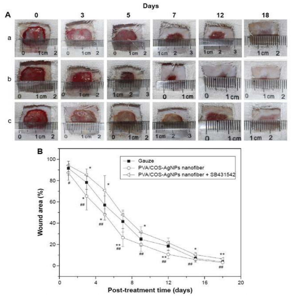
    [40] Li CW, Wang Q, Li J, et al. (2016) Silver nanoparticles/chitosan oligosaccharide/poly(vinyl alcohol) nanofiber promotes wound healing by activating TGFβ1/Smad signaling pathway. Int J Nanomedicine 11: 373-387.
    [41] Liu M, Shen Y, Ao P, et al. (2014) The improvement of hemostatic and wound healing property of chitosan by halloysite nanotubes. RSC Adv 4: 23540-23553.
    [42] Mahdavi M, Mahmoudi N, Anaran FR, et al. (2016) Electrospinning of nanodiamond-modified polysaccharide nanofibers with physico-mechanical properties close to natural skins. Mar Drugs 14: 128. doi: 10.3390/md14070128
    [43] Georgii JL, Amadeu TP, Seabra AB, et al. (2011). Topical S-nitrosoglutathione-releasing hydrogel improves healing of rat ischemic wounds. J Tissue Eng Regen Med 5: 612-619.
    [44] Zhou X, Wang H, Zhang J, et al. (2017) Functional poly(ε-caprolactone)/chitosan dressings with nitric oxide-releasing property improve wound healing. Acta Biomater 54: 128-137.
    [45] Veleirinho B, Coelho DS, Dias PF, et al. (2012) Nanofibrous poly(3-hydroxybutyrate-co-3-hydroxyvalerate)/chitosan scaffolds for skin regeneration. Int J Biol Macromolec 51: 343-350.
    [46] Archana D, Dutta J, Dutta PK (2013) Evaluation of chitosan nano dressing for wound healing: Characterization, in vitro and in vivo studies. Int J Biol Macromolec 57: 193-203.
    [47] Cao H, Chen MM, Liu Y, et al. (2015) Fish collagen-based scaffold containing PLGA microspheres for controlled growth factor delivery in skin tissue engineering. Colloids Surf B Biointerfaces 136: 1098-1106.
    [48] Gharatape A, Milani M, Rasta SH, et al. (2016) A novel strategy for low level laser-induced plasmonic photothermal therapy: the efficient bactericidal effect of biocompatible AuNPs@(PNIPAAM-co-PDMAEMA, PLGA and chitosan). RSC Adv 6: 110499-110510.
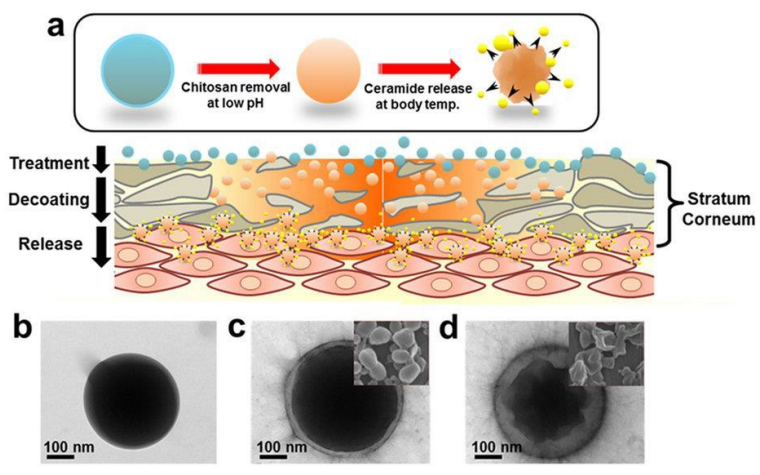
    [49] Jung SM, Yoon GH, Lee HC, et al. (2015) Thermodynamic insights and conceptual design of skin sensitive chitosan coated ceramide/PLGA nanodrug for regeneration of Stratum corneum on atopic dermatitis. Sci Rep 5: 18089.
    [50] Seabra AB, Kitice NA, Pelegrino MT, et al. (2015) Nitric oxide-releasing polymeric nanoparticles against Trypanosoma cruzi. J Phys: Conf Series 617: 012020.
    [51] Seabra AB, Duran N (2012) Nanotechnology allied to nitric oxide release materials for dermatological applications. Curr Nanosci 8: 520-525.
    [52] Seabra AB, Duran N (2017) Nanoparticulated nitric oxide donors and their biomedical applications. Mini Rev Med Chem 17: 216-223.
    [53] Han G, Martinez LR, Mihu MR, et al. (2009) Nitric oxide releasing nanoparticles are therapeutic for Staphylococcus aureus abscesses in a murine model of infection. PLoS One 4: e7804.
    [54] Shome S, Das TA, Choudhury MD, et al. (2016) Curcumin as potential therapeutic natural product: a nanobiotechnological perspective. J Pharm Pharmacol 68: 1481-1500.
    [55] Karri VV, Kuppusamy G, Talluri SV, et al. (2016) Curcumin loaded chitosan nanoparticles impregnated into collagen-alginate scaffolds for diabetic wound healing. Int J Biol Macromol 93: 1519-1529.
    [56] SeabraAB, Pankotai E, Feher M, et al. (2007) S-nitrosoglutathione-containing hydrogel increases dermal blood flow in streptozotocin-induced diabetic rats. Br J Dermatol 156: 814-818.
    [57] Lin YH, Lin JH, Hong YS (2017). Development of chitosan/poly-g-glutamic acid/pluronic/curcumin nanoparticles in chitosan dressings for wound regeneration. J Biomed Mater Res Part B 105B: 81-90.
    [58] Lin YH, Lin JH, Li TS, et al. (2016) Dressing with epigallocatechin gallate nanoparticles for wound regeneration. Wound Repair Regen 24: 287-301.
    [59] Nawaz A, Wong TW (2017) Microwave as skin permeation enhancer for transdermal drugdelivery of chitosan-5-fluorouracil nanoparticles. Carbohydr Polym 157: 906-919.
    [60] Piras AM, Maisetta G, SandreschiS, et al. (2015) Chitosan nanoparticles loaded with the antimicrobial peptide temporin B exert a long-term antibacterial activity in vitroagainst clinical isolates of Staphylococcus epidermidis. Front Microbiol 6: 372.
    [61] Ramasamy T, Kim JO, Yong CS, et al. (2015) Novel core–shell nanocapsules for the tunable delivery of bioactive rhEGF: Formulation, characterization and cytocompatibility studies. J Biomater Tissue Eng 5: 730-743.
    [62] Romić MD, Klarić MŠ, Lovrić J, et al. (2016) Melatonin-loaded chitosan/Pluronic® F127 microspheres as in situforming hydrogel: An innovative antimicrobial wound dressing. Eur J Pharm Biopharm 107: 67-79.
    [63] Abureesh MA, Oladipo AA, Gazi M (2016) Facile synthesis of glucose-sensitive chitosan-poly(vinyl alcohol) hydrogel: Drug release optimization and swelling properties. Int J Biol Macromol 90: 75-80.
    [64] Zhao X, Zou X, Ye L (2016) Controlled pH-and glucose-responsive drug release behavior of cationic chitosan based nano-composite hydrogels by using graphene oxide as drug nanocarrier. J Ind Eng Chem: 1-10.
    [65] Neufeld L, Bianco-Peled H (2017) Pectin–chitosan physical hydrogels as potential drug delivery vehicles. Int J Biol Macromol 101: 852-861.
    [66] Rogina A, Ressler A, Matic I, et al. (2017) Cellular hydrogels based on pH-responsive chitosan-hydroxyapatite system. Carbohydr Polym 166: 173-182.
    [67] Sapru S, Ghosh AK, Kundu SC (2017) Non-immunogenic, porous and antibacterial chitosan and Antheraea mylitta silk sericin hydrogels as potential dermal substitute. Carbohydr Polym 167: 196-209.
    [68] Wahid F, Wang HS, Zhong C, et al. (2017) Facile fabrication of moldable antibacterial carboxymethyl chitosan supramolecular hydrogels cross-linked by metal ions complexation. Carbohydr Polym 165: 455-461.
    [69] Yu S, Zhang X, Tan G, et al. (2017) A novel pH-induced thermosensitive hydrogel composed of carboxymethyl chitosan and poloxamer cross-linked by glutaraldehyde for ophthalmic drug delivery. Carbohydr Polym 155: 208-217.
    [70] Mohan N, Mohanan PV, Sabareeswaran A (2017) Chitosan-hyaluronic acid hydrogel for cartilage repair. Int J Biol Macromol.
    [71] Mozalewska W, Czechowska-Biskup R, Olejnik AK, et al. (2017) Chitosan-containing hydrogel wound dressings prepared by radiation technique. Radiat Phys Chem134: 1-7.
    [72] Croisier F, Jérôme C (2013) Chitosan-based biomaterials for tissue engineering. Eur Polym J 49: 780-792.
    [73] Carvalho IC, Mansur HS (2017) Engineered 3D-scaffolds of photocrosslinked chitosan-gelatin hydrogel hybrids for chronic wound dressings and regeneration. Mater Sci 93: 1519-1529.
    [74] Mohan N, Mohanan PV, Sabareeswaran A (2017) Chitosan-hyaluronic acid hydrogel for cartilage repair. Int J Biol Macromol.
    [75] Mozalewska W, Czechowska-Biskup R, Olejnik AK, et al. (2017) Chitosan-containing hydrogel wound dressings prepared by radiation technique. Radiat Phys Chem 134: 1-7.
    [76] Giri TK, Thakur A, Alexander A, et al. (2012) Modified chitosan hydrogels as drug delivery and tissue engineering systems: present status and applications. Acta Pharm Sin B 2: 439-449.
    [77] Santos JCC, Mansur AAP, Mansur HS (2013) One-step biofunctionalization of quantum dots with chitosan and n-palmitoyl chitosan for potential biomedical applications. Molecules 18: 6550-6572. doi: 10.3390/molecules18066550
    [78] Medeiros FGLB, Mansur AAP, Chagas P, et al. (2015) O-carboxymethyl functionalization of chitosan: Complexation and adsorption of Cd (II) and Cr (VI) as heavy metal pollutant ions. React Funct Polym 97: 37-47.
    [79] Yu P, Bao R-Y, Shi X-J, et al. (2017) Self-assembled high-strength hydroxyapatite/graphene oxide/chitosan composite hydrogel for bone tissue engineering. Carbohydr Polym 155: 507-515.
    [80] Liu X, Chen Y, Huang Q, et al. (2014) A novel thermo-sensitive hydrogel based on thiolated chitosan/ hydroxyapatite/beta-glycerophosphate. Carbohydr Polym 110: 62-69.
    [81] Song K, Li L, Yan X, et al. (2017) Characterization of human adipose tissue-derived stem cells in vitro culture and in vivo differentiation in a temperature-sensitive chitosan/B- glycerophosphate/collagen hybrid hydrogel. Mater Sci Eng C 70: 231-240.
    [82] Bao Z, Jiang C, Wang Z, et al. (2017) The influence of solvent formulations on thermosensitive hydroxybutyl chitosan hydrogel as a potential delivery matrix for cell therapy. Carbohydr Polym 170: 80-88.
    [83] Zhang Y, Dang Q, Liu C, et al. (2017) Synthesis, characterization, and evaluation of poly(aminoethyl) modified chitosan and its hydrogel used as antibacterial wound dressing. Int J Biol Macromol 102: 457-467.
    [84] Rabea EI, Badawy MET, Stevens C V, et al. (2003) Chitosan as antimicrobial agent: Applications and mode of action. Biomacromolecules 4: 1457-1465.
    [85] Zakrzewska A, Boorsma A, Delneri D, et al. (2007) Cellular processes and pathways that protect Saccharomyces cerevisiae cells against the plasma membrane-perturbing compound chitosan. Eukaryot Cell 6: 600-608.
    [86] Song Y, Zhang D, Lv Y, et al. (2016) Microfabrication of a tunable collagen/alginate-chitosan hydrogel membrane for controlling cell-cell interactions. Carbohydr Polym 153 :652-662.
    [87] Dang Q, Liu K, Zhang Z, et al. (2017) Fabrication and evaluation of thermosensitivechitosan/collagen/α, β-glycerophosphate hydrogels for tissue regeneration. Carbohydr Polym 167: 145-157.
    [88] Heris HK, Latifi N, Vali H, et al (2015) Investigation of Chitosan-glycol/glyoxal as an injectable biomaterial for vocal fold tissue engineering. Procedia Eng 110: 143-150.
    [89] Yap LS, Yang MC (2016) Evaluation of hydrogel composing of Pluronic F127 and carboxymethyl hexanoyl chitosan as injectable scaffold for tissue engineering applications. Colloids Surf B 146: 204-211.
    [90] Malli S, Bories C, Pradines B, et al. (2017) In situ forming Pluronic® F127/chitosan hydrogel limits metronidazole transmucosal absorption. Eur J Pharm Biopharm 112: 143-147.
    [91] Molina MM, Seabra AB, de Oliveira MG, et al. (2013) Nitric oxide donor superparamagnetic ironoxide nanoparticles. Mater Sci Eng C Mater Biol Appl 33: 746-751.
    [92] Ong SY, Wu J, Moochhala SM, et al. (2008) Development of a chitosan-based wound dressing with improved hemostatic and antimicrobial properties. Biomaterials 29: 4323-4332.
    [93] Zhou Y, Zhao Y, Wang L, et al. (2012) Radiation synthesis and characterization of nanosilver/gelatin/carboxymethyl chitosan hydrogel. Radiat Phys Chem 81: 553-560.
    [94] Sudheesh KPT, Lakshmanan VK, Anilkumar TV, et al. (2012) Flexible and microporous chitosan hydrogel/nano ZnO composite bandages for wound dressing: In vitroand in vivoevaluation. ACS Appl Mater Interfaces 4: 2618-2629.
    [95] Yang JA, Yeom J, Hwang BW, et al. (2014) In situ-forming injectable hydrogels for regenerative medicine. Prog Polym Sci 39: 1973-1986.
    [96] Hoffman AS (2012) Hydrogels for biomedical applications. Adv Drug DelivRev 64: 18-23.
    [97] Cheng NC, Lin WJ, Ling TY, et al. (2017) Sustained release of adipose-derived stem cells by thermosensitive chitosan/gelatin hydrogel for therapeutic angiogenesis. Acta Biomater 51: 258-267.
    [98] Zhang D, Zhou W, Wei B, et al. (2015) Carboxyl-modified poly(vinyl alcohol)-crosslinked chitosan hydrogel films for potential wound dressing. Carbohydr Polym 125: 189-199.
    [99] Duran N, Duran M, de Jesus MB, et al. (2016) Silver nanoparticles: A new view on mechanistic aspects on antimicrobial activity. Nanomedicine 12: 789-799.
  • Reader Comments
  • © 2017 the Author(s), licensee AIMS Press. This is an open access article distributed under the terms of the Creative Commons Attribution License (http://creativecommons.org/licenses/by/4.0)
通讯作者: 陈斌, bchen63@163.com
  • 1. 

    沈阳化工大学材料科学与工程学院 沈阳 110142

  1. 本站搜索
  2. 百度学术搜索
  3. 万方数据库搜索
  4. CNKI搜索

Metrics

Article views(8780) PDF downloads(1669) Cited by(16)

Other Articles By Authors

/

DownLoad:  Full-Size Img  PowerPoint
Return
Return

Catalog