To overcome the problem of easily falling into local extreme values of the whale swarm algorithm to solve the material emergency dispatching problem with changing road conditions, an improved whale swarm algorithm is proposed. First, an improved scan and Clarke-Wright algorithm is used to obtain the optimal vehicle path at the initial time. Then, the group movement strategy is designed to generate offspring individuals with an improved quality for refining the updating ability of individuals in the population. Finally, in order to maintain population diversity, a different weights strategy is used to expand individual search spaces, which can prevent individuals from prematurely gathering in a certain area. The experimental results show that the performance of the improved whale swarm algorithm is better than that of the ant colony system and the adaptive chaotic genetic algorithm, which can minimize the cost of material distribution and effectively eliminate the adverse effects caused by the change of road conditions.
Citation: Huawei Jiang, Shulong Zhang, Tao Guo, Zhen Yang, Like Zhao, Yan Zhou, Dexiang Zhou. Improved whale swarm algorithm for solving material emergency dispatching problem with changing road conditions[J]. Mathematical Biosciences and Engineering, 2023, 20(8): 14414-14437. doi: 10.3934/mbe.2023645
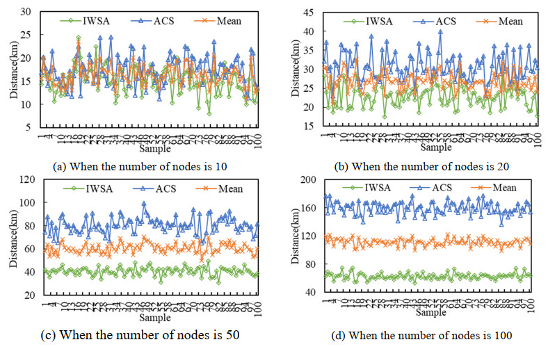
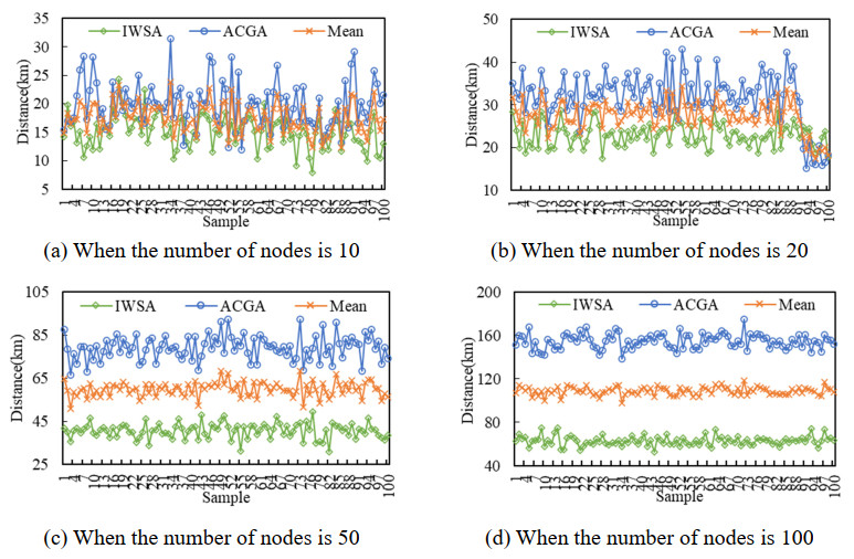
To overcome the problem of easily falling into local extreme values of the whale swarm algorithm to solve the material emergency dispatching problem with changing road conditions, an improved whale swarm algorithm is proposed. First, an improved scan and Clarke-Wright algorithm is used to obtain the optimal vehicle path at the initial time. Then, the group movement strategy is designed to generate offspring individuals with an improved quality for refining the updating ability of individuals in the population. Finally, in order to maintain population diversity, a different weights strategy is used to expand individual search spaces, which can prevent individuals from prematurely gathering in a certain area. The experimental results show that the performance of the improved whale swarm algorithm is better than that of the ant colony system and the adaptive chaotic genetic algorithm, which can minimize the cost of material distribution and effectively eliminate the adverse effects caused by the change of road conditions.

| [1] |
L. Zhou, X. Wu, Z. Xu, H. Fujita, Emergency decision making for natural disasters: An overview, Int. J. Disaster Risk Reduct., 27 (2018), 567–576. https://doi.org/10.1016/j.ijdrr.2017.09.037 doi: 10.1016/j.ijdrr.2017.09.037

|
| [2] |
M. M. Boer, V. R. de Dios, R. A. Bradstock, Unprecedented burn area of Australian mega forest fires, Nat. Clim. Chang., 10 (2020), 171–172. https://doi.org/10.1038/s41558-020-0716-1 doi: 10.1038/s41558-020-0716-1
|
| [3] |
S. R. Stewart, The 2020 atlantic hurricane season: The most active season on record, Weatherwise, 74 (2021), 44–51. https://doi.org/10.1080/00431672.2021.1953906 doi: 10.1080/00431672.2021.1953906
|
| [4] |
Y. Yin, F. Wang, P. Sun, Landslide hazards triggered by the 2008 Wenchuan earthquake, Sichuan, China, Landslides, 6 (2009), 139–152. https://doi.org/10.1007/s10346-009-0148-5 doi: 10.1007/s10346-009-0148-5
|
| [5] |
X. Guo, J. Cheng, C. Yin, Q. Li, R. Chen, J. Fang, The extraordinary Zhengzhou flood of 7/20, 2021: How extreme weather and human response compounding to the disaster, Cities, 134 (2023), 104168. https://doi.org/10.1016/j.cities.2022.104168 doi: 10.1016/j.cities.2022.104168
|
| [6] |
A. Expósito, J. Brito, J. A. Moreno, C. Expósito-Izquierdo, Quality of service objectives for vehicle routing problem with time windows, Appl. Soft. Comput., 84 (2019), 105707. https://doi.org/10.1016/j.asoc.2019.105707 doi: 10.1016/j.asoc.2019.105707
|
| [7] |
Y. Qi, Y. Cai, H. Cai, H. Huang, Discrete bat algorithm for vehicle routing problem with time window, Acta Electron. Sin., 46 (2018), 672–679. https://doi.org/10.3969/j.issn.0372-2112.2018.03.024 doi: 10.3969/j.issn.0372-2112.2018.03.024
|
| [8] |
H. Tang, B. Wu, W. Hu, C. Kang, Earthquake emergency resource multiobjective schedule algorithm based on particle swarm optimization, J. Electron. Inf. Technol., 42 (2020), 737–745. https://doi.org/10.11999/JEIT190277 doi: 10.11999/JEIT190277
|
| [9] |
H. C. W. Lau, T. M. Chan, W. T. Tsui, W. K. Pang, Application of genetic algorithms to solve the multidepot vehicle routing problem, IEEE Trans. Autom. Sci. Eng., 7 (2010), 383–392. https://doi.org/10.1109/TASE.2009.2019265 doi: 10.1109/TASE.2009.2019265
|
| [10] |
Z. Zhang, H. Qin, Y. Li, Multi-objective optimization for the vehicle routing problem with outsourcing and profit balancing, IEEE Trans. Intell. Transp. Syst., 21 (2020), 1987–2001. https://doi.org/10.1109/TITS.2019.2910274 doi: 10.1109/TITS.2019.2910274
|
| [11] |
Y. Yi, Y. Cai, W. Dong, X. Lin, Improved ITO algorithm for multiobjective real-time vehicle routing problem with customers' satisfaction, Acta Electron. Sin., 43 (2015), 2053–2061. https://doi.org/10.3969/j.issn.0372-2112.2015.10.026 doi: 10.3969/j.issn.0372-2112.2015.10.026
|
| [12] |
G. Kim, Y. S. Ong, T. Cheong, P. S. Tan, Solving the dynamic vehicle routing problem under traffic congestion, IEEE Trans. Intell. Transp. Syst., 17 (2016), 2367–2380. https://doi.org/10.1109/TITS.2016.2521779 doi: 10.1109/TITS.2016.2521779
|
| [13] |
G. Ghiani, F. Guerriero, G. Laporte, R. Musmanno, Real-time vehicle routing: Solution concepts, algorithms and parallel computing strategies, Eur. J. Oper. Res., 151 (2003), 1–11. https://doi.org/10.1016/S0377-2217(02)00915-3 doi: 10.1016/S0377-2217(02)00915-3
|
| [14] |
H. N. Psaraftis, M. Wen, C. A. Kontovas, Dynamic vehicle routing problems: Three decades and counting, Networks, 67 (2016), 3–31. https://doi.org/10.1002/net.21628 doi: 10.1002/net.21628
|
| [15] |
M. Zhang, N. Wang, Z. He, Z. Yang, Y. Guan, Bi-objective vehicle routing for hazardous materials transportation with actual load dependent risks and considering the risk of each vehicle, IEEE Trans. Eng. Manage., 66 (2019), 429–442. https://doi.org/10.1109/TEM.2018.2832049 doi: 10.1109/TEM.2018.2832049
|
| [16] |
X. Zhou, L. Wang, K. Zhou, X. Huang, Research progress and development trend of dynamic vehicle routing problem, Control Decis., 34 (2019), 449–458. https://doi.org/10.13195/j.kzyjc.2018.1304 doi: 10.13195/j.kzyjc.2018.1304
|
| [17] |
Y. Yu, S. Wang, J. Wang, M. Huang, A branch-and-price algorithm for the heterogeneous fleet green vehicle routing problem with time windows, Transp. Res. Part B: Methodol., 122 (2019), 511–527. https://doi.org/10.1016/j.trb.2019.03.009 doi: 10.1016/j.trb.2019.03.009
|
| [18] |
N. Azi, M. Gendreau, J. Potvin, An exact algorithm for a single-vehicle routing problem with time windows and multiple routes, Eur. J. Oper. Res., 178 (2007), 755–766. https://doi.org/10.1016/j.ejor.2006.02.019 doi: 10.1016/j.ejor.2006.02.019
|
| [19] |
W. Yang, L. Ke, D. Z. W. Wang, J. S. L. Lam, A branch-price-and-cut algorithm for the vehicle routing problem with release and due dates, Transp. Res. Part B: Logist. Transp. Rev., 145 (2021), 102167. https://doi.org/10.1016/j.tre.2020.102167 doi: 10.1016/j.tre.2020.102167
|
| [20] |
H. Zhang, Q. Zhang, L. Ma, Z. Zhang, Y. Liu, A hybrid ant colony optimization algorithm for a multi-objective vehicle routing problem with flexible time windows, Inf. Sci., 490 (2019), 166–190. https://doi.org/10.1016/j.ins.2019.03.070 doi: 10.1016/j.ins.2019.03.070
|
| [21] |
J. Luo, X. Li, M. Chen, Improved shuffled frog leaping algorithm for solving CVRP, J. Electron. Inf. Technol., 33 (2011), 429–434. https://doi.org/10.3724/SP.J.1146.2010.00328 doi: 10.3724/SP.J.1146.2010.00328
|
| [22] |
R, Hu, Y. Li, B. Qian, H. Jin, F. Xiang, An enhanced ant colony algorithm combined with clustering decomposition for complex green vehicle routing problem, Acta Autom. Sin., 48 (2022), 3006–3023. https://doi.org/10.16383/j.aas.c190872 doi: 10.16383/j.aas.c190872
|
| [23] |
M. Desrochers, J. Desrosiers, M. Solomon, A new optimization algorithm for the vehicle routing problem with time windows, Oper. Res., 40 (1992), 342–354. https://doi.org/10.1287/opre.40.2.342 doi: 10.1287/opre.40.2.342
|
| [24] |
M. M. S. Abdulkader, Y. Gajpal, T. Y. ElMekkawy, Hybridized ant colony algorithm for the multi compartment vehicle routing problem, Appl. Soft. Comput., 37 (2015), 196–203. https://doi.org/10.1016/j.asoc.2015.08.020 doi: 10.1016/j.asoc.2015.08.020
|
| [25] | H. Wu, X. Chen, Q. Mao, Q. Zhang, S. Zhang, Improved ant colony algorithm based on natural selection strategy for solving TSP problem, J. Commun., 34 (2013), 165–170. |
| [26] |
I. Sung, T. Lee, Optimal allocation of emergency medical resources in a mass casualty incident: Patient prioritization by column generation, Eur. J. Oper. Res., 252 (2016), 623–634. https://doi.org/10.1016/j.ejor.2016.01.028 doi: 10.1016/j.ejor.2016.01.028
|
| [27] |
B. Balcik, B. M. Beamon, K. Smilowitz, Last mile distribution in humanitarian relief, J. Intel. Transp. Syst., 12 (2008), 51–63. https://doi.org/10.1080/15472450802023329 doi: 10.1080/15472450802023329
|
| [28] |
B. Vitoriano, M. T. Ortuño, G. Tirado, J. Montero, A multi-criteria optimization model for humanitarian aid distribution, J. Glob. Optim., 51 (2011), 189–208. https://doi.org/10.1007/s10898-010-9603-z doi: 10.1007/s10898-010-9603-z
|
| [29] |
G. Zhang, Y. Wang, Z. Su, J. Jiang, Modeling and solving multi-objective allocation-scheduling of emergency relief supplies, Control Decis., 32 (2017), 86–92. https://doi.org/10.13195/j.kzyjc.2015.1518 doi: 10.13195/j.kzyjc.2015.1518
|
| [30] |
D. Chen, F. Ding, Y. Huang, D. Sun, Multi-objective optimisation model of emergency material allocation in emergency logistics: A view of utility, priority and economic principles, Int. J. Emerg. Manage., 14 (2018), 233–253. https://doi.org/10.1504/IJEM.2018.094236 doi: 10.1504/IJEM.2018.094236
|
| [31] |
F. Wex, G. Schryen, S. Feuerriegel, D. Neumann, Emergency response in natural disaster management: Allocation and scheduling of rescue units, Eur. J. Oper. Res., 235 (2014), 697–708. https://doi.org/10.1016/j.ejor.2013.10.029 doi: 10.1016/j.ejor.2013.10.029
|
| [32] |
X. Song, J. Wang, C. Chang, Nonlinear continuous consumption emergency material dispatching problem, J. Syst. Eng., 32 (2017), 163–176. https://doi.org/10.13383/j.cnki.jse.2017.02.003 doi: 10.13383/j.cnki.jse.2017.02.003
|
| [33] |
C. Qu, J. Wang, J. Huang, M. He, Dynamic emergency materials distribution optimization with timeliness and fairness objective for post-earthquake emergency rescue, Chin. J. Manage. Sci., 26 (2018), 178–187. https://doi.org/10.16381/j.cnki.issn1003-207x.2018.06.018 doi: 10.16381/j.cnki.issn1003-207x.2018.06.018
|
| [34] |
B. Fleischmann, S. Gnutzmann, E. Sandvoß, Dynamic vehicle routing based on online traffic information, Transp. Sci., 38 (2004), 420–433. https://doi.org/10.1287/trsc.1030.0074 doi: 10.1287/trsc.1030.0074
|
| [35] | Y. Li, Z. Gao, J. Li, Vehicle routing problem in dynamic urban traffic network, in 2011 8th International Conference on Service Systems and Service Management (ICSSSM), (2011), 1257–1262. https://doi.org/10.1109/ICSSSM.2011.5959534 |
| [36] |
I. Okhrin, K. Richter, Vehicle routing problem with real-time travel times, Int. J. Veh. Inf. Commun. Syst., 2 (2009), 59–77. https://doi.org/10.1504/IJVICS.2009.027746 doi: 10.1504/IJVICS.2009.027746
|
| [37] |
Y. Li, Z. Y. Gao, J. Li, Vehicle routing optimization in urban dynamic network based on real-time traffic information, Syst. Eng. Theory Pract., 33 (2013), 1813–1819. https://doi.org/10.3969/j.issn.1000-6788.2013.07.022 doi: 10.3969/j.issn.1000-6788.2013.07.022
|
| [38] |
J. Zhang, J. Li, Z. Liu, Multiple-resource and multiple-depot emergency response problem considering secondary disasters, Expert Syst. Appl., 39 (2012), 11066–11071. https://doi.org/10.1016/j.eswa.2012.03.016 doi: 10.1016/j.eswa.2012.03.016
|
| [39] |
E. Queiroga, Y. Frota, R. Sadykov, A. Subramanian, E. Uchoa, T. Vidal, On the exact solution of vehicle routing problems with backhauls, Eur. J. Oper. Res., 287 (2020), 76–89. https://doi.org/10.1016/j.ejor.2020.04.047 doi: 10.1016/j.ejor.2020.04.047
|
| [40] |
X. Xiang, Y. Tian, X. Zhang, J. Xiao, Y. Jin, A pairwise proximity learning-based ant colony algorithm for dynamic vehicle routing problems, IEEE Trans. Intell. Transp. Syst., 23 (2022), 5275–5286. https://doi.org/10.1109/TITS.2021.3052834 doi: 10.1109/TITS.2021.3052834
|
| [41] |
F. Wang, Z. Pei, L. Dong, J. Ma, Emergency resource allocation for multi-period post-disaster using multi-objective cellular genetic algorithm, IEEE Access, 8 (2020), 82255–82265. https://doi.org/10.1109/ACCESS.2020.2991865 doi: 10.1109/ACCESS.2020.2991865
|
| [42] |
L. Zhang, H. Zhang, D. Liu, Y. Lu, Particle swarm algorithm for solving emergency material dispatch considering urgency, J. Syst. Simul., 34 (2022), 1988–1998. https://doi.org/10.16182/j.issn1004731x.joss.21-0362 doi: 10.16182/j.issn1004731x.joss.21-0362
|
| [43] | B. Zeng, L. Gao, X. Li, Whale swarm algorithm for function optimization, in International Conference on Intelligent Computing, 10361 (2017), 624–639. https://doi.org/10.1007/978-3-319-63309-1_55 |
| [44] |
J. Dong, C. Ye, Collaborative optimization of interval number reentrant hybrid flow shop scheduling and preventive maintenance, Control Decis., 36 (2021), 2599–2608. https://doi.org/10.13195/j.kzyjc.2020.0973 doi: 10.13195/j.kzyjc.2020.0973
|
| [45] |
C. Zhang, J. Tan, K. Peng, L. Gao, W. Shen, K. Lian, A discrete whale swarm algorithm for hybrid flow-shop scheduling problem with limited buffers, Rob. Comput. Integr. Manuf., 68 (2021), 102081. https://doi.org/10.1016/j.rcim.2020.102081 doi: 10.1016/j.rcim.2020.102081
|
| [46] |
H. K. Chen, C. F. Hsueh, M. S. Chang, The real-time time-dependent vehicle routing problem, Transp. Res. Part E: Logist. Transp. Rev., 42 (2006), 383–408. https://doi.org/10.1016/j.tre.2005.01.003 doi: 10.1016/j.tre.2005.01.003
|
| [47] |
G. Clarke, J. W. Wright, Scheduling of vehicles from a central depot to a number of delivery points, Oper. Res., 12 (1964), 568–581. https://doi.org/10.1287/opre.12.4.568 doi: 10.1287/opre.12.4.568
|
| [48] |
S. Hougardy, F. Zaiser, X. Zhong, The approximation ratio of the 2-Opt heuristic for the metric traveling salesman problem, Oper. Res. Lett., 48 (2020), 401–404. https://doi.org/10.1016/j.orl.2020.05.007 doi: 10.1016/j.orl.2020.05.007
|
| [49] | J. Sripriya, A. Ramalingam, K. Rajeswari, A hybrid genetic algorithm for vehicle routing problem with time windows, in 2015 International Conference on Innovations in Information, Embedded and Communication Systems (ICⅡECS), (2015), 1–4. https://doi.org/10.1109/ICⅡECS.2015.7193072 |
| [50] | D. Huang, X. Yan, X. Chu, Z. Mao, An adaptive algorithm for dynamic vehicle routing problem based on real time traffic information, in ICTIS 2011: Multimodal Approach to Sustained Transportation System Development: Information, Technology, Implementation, (2011), 1736–1744. https://doi.org/10.1061/41177(415)220 |
| [51] | Y. Chen, X. Hu, G. Ye. Research on related vehicle routing problem for single distribution center based on dynamic constraint, in 2013 Ninth International Conference on Computational Intelligence and Security, (2013), 76–79. https://doi.org/10.1109/CIS.2013.23 |
Figures(7) / Tables(5)

Huawei Jiang, Shulong Zhang, Tao Guo, Zhen Yang, Like Zhao, Yan Zhou, Dexiang Zhou. Improved whale swarm algorithm for solving material emergency dispatching problem with changing road conditions[J]. Mathematical Biosciences and Engineering, 2023, 20(8): 14414-14437. doi: 10.3934/mbe.2023645


 DownLoad: