Currently, machine learning methods have been utilized to realize the early detection of Parkinson's disease (PD) by using voice signals. Because the vocal system of each person is unique, and the same person's pronunciation can be different at different times, the training samples used in machine learning become very different from the speech signal of the patient to be diagnosed, frequently resulting in poor diagnostic performance. On this account, this paper presents a new intelligent personalized diagnosis method (PDM) for Parkinson's disease. The method was designed to begin with constructing new training data by assigning the best classifier to each training sample composed of features from the speech signals of patients. Subsequently, a meta-classifier was trained on the new training data. Finally, for the signal of each test patient, the method used the meta-classifier to select the most appropriate classifier, followed by adopting the selected classifier to classify the signal so that the more accurate diagnosis result of the test patient can be obtained. The novelty of the proposed method is that the proposed method uses different classifiers to perform the diagnosis of PD for diversified patients, whereas the current method uses the same classifier to diagnose all patients to be tested. Results of a large number of experiments show that PDM not only improves the performance but also exceeds the existing methods in speed.
Citation: Pengcheng Wen, Yuhan Zhang, Guihua Wen. Intelligent personalized diagnosis modeling in advanced medical system for Parkinson's disease using voice signals[J]. Mathematical Biosciences and Engineering, 2023, 20(5): 8085-8102. doi: 10.3934/mbe.2023351
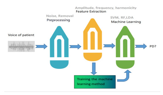
Currently, machine learning methods have been utilized to realize the early detection of Parkinson's disease (PD) by using voice signals. Because the vocal system of each person is unique, and the same person's pronunciation can be different at different times, the training samples used in machine learning become very different from the speech signal of the patient to be diagnosed, frequently resulting in poor diagnostic performance. On this account, this paper presents a new intelligent personalized diagnosis method (PDM) for Parkinson's disease. The method was designed to begin with constructing new training data by assigning the best classifier to each training sample composed of features from the speech signals of patients. Subsequently, a meta-classifier was trained on the new training data. Finally, for the signal of each test patient, the method used the meta-classifier to select the most appropriate classifier, followed by adopting the selected classifier to classify the signal so that the more accurate diagnosis result of the test patient can be obtained. The novelty of the proposed method is that the proposed method uses different classifiers to perform the diagnosis of PD for diversified patients, whereas the current method uses the same classifier to diagnose all patients to be tested. Results of a large number of experiments show that PDM not only improves the performance but also exceeds the existing methods in speed.

| [1] |
S. Singh, W. Xu, Robust detection of Parkinson's disease using harvested smartphone voice data: a telemedicine approach, Telemed. e-Health, 26 (2020), 327–334. https://doi.org/10.1089/tmj.2018.0271 doi: 10.1089/tmj.2018.0271

|
| [2] |
A. Tsanas, M. Little, P. McSharry, L. Ramig, Accurate telemonitoring of Parkinson's disease progression by non-invasive speech tests, Nat. Preced., 2009 (2009). https://doi.org/10.1038/npre.2009.3920.1 doi: 10.1038/npre.2009.3920.1
|
| [3] |
T. L. Yang, C. H. Lin, W. L. Chen, H. Y. Lin, C. S. Su, C. K. Liang, Hash transformation and machine learning-based decision-making classifier improved the accuracy rate of automated Parkinson's disease screening, IEEE Trans. Neural Syst. Rehabil. Eng., 28 (2020), 72–82. https://doi.org/10.1109/TNSRE.2019.2950143 doi: 10.1109/TNSRE.2019.2950143
|
| [4] |
O. Y. Chen, F. Lipsmeier, H. Phan, J. Prince, K. I. Taylor, C. Gossens, et al., Building a machine-learning framework to remotely assess Parkinson's disease using smartphones, IEEE Trans. Biomed. Eng., 67 (2020), 3491–3500. https://doi.org/10.1109/TBME.2020.2988942 doi: 10.1109/TBME.2020.2988942
|
| [5] |
T. Tuncer, S. Dogan, U. R. Acharya, Automated detection of Parkinson's disease using minimum average maximum tree and singular value decomposition method with vowels, Biocybern. Biomed. Eng., 40 (2020), 211–220. https://doi.org/10.1016/j.bbe.2019.05.006 doi: 10.1016/j.bbe.2019.05.006
|
| [6] |
S. A. Mostafa, A. Mustapha, M. A. Mohammed, R. I. Hamed, N. Arunkumar, S. H. Khaleefah, et al., Examining multiple feature evaluation and classification methods for improving the diagnosis of Parkinson's disease, Cognit. Syst. Res., 54 (2019), 90–99. https://doi.org/10.1016/j.cogsys.2018.12.004 doi: 10.1016/j.cogsys.2018.12.004
|
| [7] |
I. EI. Maachi, G. Bilodeau, W. Bouachir, Deep 1D-Convnet for accurate Parkinson disease detection and severity prediction from gait, Expert Syst. Appl., 143 (2020), 113075. https://doi.org/10.1016/j.eswa.2019.113075 doi: 10.1016/j.eswa.2019.113075
|
| [8] |
S. Aich, P. M. Pradhan, S. Chakraborty, H. Kim, M. Joo, J. Park, et al., Design of a machine learning-assisted wearable accelerometer-based automated system for studying the effect of dopaminergic medicine on gait characteristics of Parkinson's patients, J. Healthcare Eng., 2020 (2020), 1823268. https://doi.org/10.1155/2020/1823268 doi: 10.1155/2020/1823268
|
| [9] |
S. Rosenblum, S. Meyer, A. Richardson, S. Hassin-Baer, Patients' self-report and handwriting performance features as indicators for suspected mild cognitive impairment in Parkinson's disease, Sensors, 22 (2022). https://doi.org/10.3390/s22020569 doi: 10.3390/s22020569
|
| [10] | Q. T. Ly, A. M. Ardi Handojoseno, M. Gilat, R. Chai, K. Martens, M. Georgiades, et al., Detection of turning freeze in Parkinson's disease based on S-transform decomposition of EEG signals, in 2017 39th Annual International Conference of the IEEE Engineering in Medicine and Biology Society, (2017), 3044–3047. https://doi.org/10.1109/EMBC.2017.8037499 |
| [11] |
Z. Y. Shu, S. J. Cui, X. Wu, P. Huang, P. P. Pang, Y. Xu, et al., Predicting the progression of Parkinson's disease using conventional MRI and machine learning: An application of radiomic biomarkers in whole-brain white matter, Magn. Reson. Med., 85 (2021), 1611–1624. https://doi.org/10.1002/mrm.28522 doi: 10.1002/mrm.28522
|
| [12] |
L. Yang, X. Chen, J. Zhang, Q. Guo, J. Zhang, X. Zou, et al., Changes in facial expressions in patients with Parkinson's disease during the phonation test and their correlation with disease severity, Comput. Speech Lang., 72 (2022). https://doi.org/10.1016/j.csl.2021.101286 doi: 10.1016/j.csl.2021.101286
|
| [13] |
J. Archila, A. Manzanera, F. Martinez, A multimodal Parkinson quantification by fusing eye and gait motion patterns, using covariance descriptors, from non-invasive computer vision, Comput. Methods Programs Biomed., 215 (2022). https://doi.org/10.1016/j.cmpb.2021.106607 doi: 10.1016/j.cmpb.2021.106607
|
| [14] | L. Gutierrez-Loaiza, W. Alfonso-Morales, Morpho-logical neural networks for Parkinson detection through speech signals, in IEEE Colombian Conference on Applications of Computational Intelligence, (2020). https://doi.org/10.1109/ColCACI50549.2020.9247918 |
| [15] |
M. G. Krokidis, G. N. Dimitrakopoulos, A. G. Vrahatis, C. Tzouvelekis, D. Drakoulis, T. P. Exarchos, et al., A sensor-based perspective in early-stage Parkinson' disease: current state and the need for machine learning processes, Sensors, 22 (2022). https://doi.org/10.3390/s22020409 doi: 10.3390/s22020409
|
| [16] | A. S. Gullapalli, V. K. Mittal, Early detection of Parkinson's disease through speech features and machine learning: a review, in ICT with Intelligent Applications, Springer nature, (2022), 203–212. https://doi.org/10.1007/978-981-16-4177-0_22 |
| [17] | R. Viswanathan, P. Khojasteh, B. Aliahmad, S. P. Arjunan, P. Kempster, K. Wong, et al., Efficiency of voice features based on consonant for detection of Parkinson's disease, in 2018 IEEE Life Sciences Conference, 2018. https://doi.org/49-52.10.1109/LSC.2018.8572266 |
| [18] |
T. Khan, L. E. Lundgren, D. G. Anderson, I. Nowak, M. Dougherty, A. Verikas, et al., Assessing Parkinson's disease severity using speech analysis in non-native speakers, Comput. Speech Lang., 61 (2020). https://doi.org/10.1016/j.csl.2019.101047 doi: 10.1016/j.csl.2019.101047
|
| [19] |
D. Gupta, A. Julka, S. Jain, T. Aggarwal, A. Khanna, N. Arunkumar, et al., Optimized cuttlefish algorithm for diagnosis of Parkinson's disease, Cognit. Syst. Res., 52 (2018). https://doi.org/10.1016/j.cogsys.2018.06.006 doi: 10.1016/j.cogsys.2018.06.006
|
| [20] | M. Pramanik, R. Pradhan, P. Nandy, Biomarkers for detection of Parkinson's disease using machine learning-A short review, in Soft Computing Techniques and Applications, Springer nature, (2020), 461–475. https://doi.org/10.1007/978-981-15-7394-1_43 |
| [21] |
A. UI Haq, J. Li, M. H. Memon, J. Khan, A. Malik, A. Ali, et al., Feature selection based on L1-norm support vector machine and effective recognition system for Parkinson's disease using voice recordings, IEEE Access, 2019 (2019), 37718–37734. https://doi.org/10.1109/ACCESS.2019.2906350 doi: 10.1109/ACCESS.2019.2906350
|
| [22] |
S. Arora, L. Baghai-Ravary, A. Tsanas, Developing a large scale population screening tool for the assessment of Parkinson' disease using telephone-quality voice, J. Acoust. Soc. Am., 145 (2019), 2871–2884. https://doi.org/10.1121/1.5100272 doi: 10.1121/1.5100272
|
| [23] |
M. Nilashi, O. Ibrahim, S. Samad, H. Ahmadi, L. Shahmoradi, E. Akbari, An analytical method for measuring the Parkinson's disease progression: a case on a Parkinson's telemonitoring dataset, Measurement, 136 (2019), 545–557. https://doi.org/10.1016/j.measurement.2019.01.014 doi: 10.1016/j.measurement.2019.01.014
|
| [24] | A. B. Soliman, M. Fares, M. M. Elhefnawi, M. Al-Hefnawy, Features selection for building an early diagnosis machine learning model for Parkinson's disease, in 2016 Third International Conference on Artificial Intelligence and Pattern Recognition, 2016. https://doi.org/10.1109/ICAIPR.2016.7585225 |
| [25] |
G. Solana-Lavalle, J. Galán-Hernández, R. Rosas-Romero, Automatic Parkinson disease detection at early stages as a pre-diagnosis tool by using classifiers and a small set of vocal features, Biocybern. Biomed. Eng., 40 (2020), 505–516. https://doi.org/10.1016/j.bbe.2020.01.003 doi: 10.1016/j.bbe.2020.01.003
|
| [26] |
M. Nilashi, H. Ahmadi, A. Sheikhtaheri, R. Naemi, R. Naemi, R. Alotaibi, et al., Remote tracking of Parkinson's disease progression using ensembles of Deep Belief Network and Self-Organizing Map, Expert Syst. Appl., 159 (2020). https://doi.org/10.1016/j.eswa.2020.113562 doi: 10.1016/j.eswa.2020.113562
|
| [27] | N. Fayyazifar, N. Samadiani, Parkinson's disease detection using ensemble techniques and genetic algorithm, in IEEE Artificial intelligence and signal processing conference, (2017), 162–165. https://doi.org/10.1109/AISP.2017.8324074 |
| [28] |
H. Kaur, A. Malhi, H. S. Pannu, Machine learning ensemble for neurological disorders, Neural Comput. Appl., 32 (2020), 12697–12714. https://doi.org/10.1007/s00521-020-04720-1 doi: 10.1007/s00521-020-04720-1
|
| [29] | S. Aich, K. Younga, K. Hui, A. Al-Absi, M. Sain, A nonlinear decision tree based classification approach to predict the Parkinson's disease using different feature sets of voice data, in International Conference on Advanced Communication Technology, (2018), 638–642. https://doi.org/10.23919/ICACT.2018.8323864 |
| [30] |
A. K. Dutta, N. M. A. Zakari, Y. Albagory, A. R. Wahab Sait, Colliding bodies optimization with machine learning based Parkinson's disease diagnosis, Comput. Syst. Sci. Eng., 44 (2023), 2195–2207. https://doi.org/10.32604/csse.2023.026461 doi: 10.32604/csse.2023.026461
|
| [31] |
G. Prema Arokia Mary, N. Suganthi, Detection of Parkinson's disease with multiple feature extraction models and darknet CNN classification, Comput. Syst. Sci. Eng., 43 (2022), 333–345. https://doi.org/10.32604/csse.2022.021164 doi: 10.32604/csse.2022.021164
|
| [32] |
R. Prashanth, S. Dutta Roy, P. K. Mandal, S. Ghosh, High-accuracy detection of early Parkinson's disease through multimodal features and machine learning, Int. J. Med. Inf., 90 (2016), 13–21. https://doi.org/10.1016/j.ijmedinf.2016.03.001 doi: 10.1016/j.ijmedinf.2016.03.001
|
| [33] |
F. Saeed, M. Al-Sarem, M. Al-Mohaimeed, A. Emara, W. Boulila, M. Alasli, et al., Enhancing Parkinson's disease prediction using machine learning and feature selection methods, Comput. Mater. Continua, 71 (2022). https://doi.org/10.32604/cmc.2022.023124 doi: 10.32604/cmc.2022.023124
|
| [34] |
P. Magesh, R. Myloth, R. Tom, An explainable machine learning model for early detection of Parkinson's disease using LIME on DaTSCAN imagery, Comput. Biol. Med., 126 (2020). https://doi.org/10.1016/j.compbiomed.2020.104041 doi: 10.1016/j.compbiomed.2020.104041
|
| [35] |
M. Hires, M. Gazda, P. Drotar, N. Pah, M. Motin, D. Kumar, Convolutional neural network ensemble for Parkinson's disease detection from voice recordings, Comput. Biol. Med., 141 (2022). https://doi.org/10.1016/j.compbiomed.2021.105021 doi: 10.1016/j.compbiomed.2021.105021
|
| [36] |
M. A. Schulz, B. Yeo, J. T. Vogelstein, J. M-Miranada, J. N. Kather, K. Kording, et al., Different scaling of linear models and deep learning in UKBiobank brain images versus machine-learning datasets, Nat. Commun., 11 (2020). https://doi.org/10.1038/s41467-020-18037-z doi: 10.1038/s41467-020-18037-z
|
| [37] |
K. Seddiki, P. Saudemont, F. Precioso, N. Ogrinc, M. Wisztorski, M. Salzet, et al., Cumulative learning enables convolutional neural network representations for small mass spectrometry data classification, Nat. Commun., 11 (2020). https://doi.org/10.1038/s41467-020-19354-z doi: 10.1038/s41467-020-19354-z
|
| [38] |
Y. Liu, Y. Li, X. Tan, P. Wang, Y. Zhang, Local discriminant preservation projection embedded ensemble learning based dimensionality reduction of speech data of Parkinson's disease, Biomed. Signal Process. Control, 63 (2021). https://doi.org/10.1016/j.bspc.2020.102165 doi: 10.1016/j.bspc.2020.102165
|
| [39] |
Y. Qiu, H. Zheng, A. Devos, H. Selby, O. Gevaert, A meta-learning approach for genomic survival analysis, Nat. Commun., 11 (2020). https://doi.org/10.1038/s41467-020-20167-3 doi: 10.1038/s41467-020-20167-3
|
| [40] |
M. R. Salmanpour, M. Shamsaei, A. Saberi, G. Hajianfar, H. Soltanian-Zadeh, A. Rahmim, Robust identification of Parkinson's disease subtypes using radiomics and hybrid machine learning, Comput. Biol. Med., 129 (2021). https://doi.org/10.1016/j.compbiomed.2020.104142 doi: 10.1016/j.compbiomed.2020.104142
|
| [41] | A. Miladinovic, M. Ajcevic, P. Busan, J. Jarmolowska, G. Silveri, S. Mezzarobba, et al., Transfer learning improves MI BCI models classification accuracy in Parkinson's disease patients, in European Signal Processing Conference, 2021. https://doi.org/10.23919/Eusipco47968.2020.9287391 |
| [42] |
Q. Yu, Y. Ma, Y. Li, Enhancing speech recognition for Parkinson's disease patient using transfer learning technique, J. Shanghai Jiaotong Univ., 27 (2022), 90–98. https://doi.org/10.1007/s12204-021-2376-3 doi: 10.1007/s12204-021-2376-3
|
| [43] |
H. Li, G. Wen, Sample awareness-based personalized facial expression recognition, Appl. Intell., 49 (2019), 2956–2969. https://doi.org/10.1007/s10489-019-01427-2 doi: 10.1007/s10489-019-01427-2
|
| [44] |
Y. Gao, Y. Cui, Deep transfer learning for reducing health care disparities arising from biomedical data inequality, Nat. Commun., 11 (2020). https://doi.org/10.1038/s41467-020-18918-3 doi: 10.1038/s41467-020-18918-3
|
| [45] |
Md. S. R. Sajal, Md. T. Ehsan, R. Vaidyanathan, S. Wang, T. Aziz, K. Mamun, Tele-monitoring Parkinson's disease using machine learning by combining tremor and voice analysis, Brain. Inf., 7 (2020). https://doi.org/10.1186/s40708-020-00113-1 doi: 10.1186/s40708-020-00113-1
|
| [46] |
L. Zahid, M. Maqsood, M. Y. Durrani, M. Bakhtyar, J. Baber, H. Jamal, et al., A spectrogram-based deep feature assisted computer-aided diagnostic system for Parkinson's disease, IEEE Access, 8 (2020). https://doi.org/10.1109/ACCESS.2020.2974008 doi: 10.1109/ACCESS.2020.2974008
|
| [47] | Y. Li, Y. Yang, S. Zhou, J. Qiao, B. Long, Deep transfer learning for search and recommendation, in Companion Proceedings of the Web Conference, (2020), 313–314. https://doi.org/10.1145/3366424.3383115 |
| [48] |
B. E. Sakar, G. Serbes, C. Okan Sakar, Analyzing the effectiveness of vocal features in early telediagnosis of Parkinson's disease, PLoS. ONE, 12 (2017), 1–18. https://doi.org/10.1371/journal.pone.0182428 doi: 10.1371/journal.pone.0182428
|
| [49] |
K. Mamun, M. Alhussein, K. Sailunaz, M. Islam, Cloud based framework for Parkinson's disease diagnosis and monitoring system for remote healthcare applications, Future Gener. Comput. Syst., 66 (2017), 36–47. https://doi.org/10.1016/j.future.2015.11.010 doi: 10.1016/j.future.2015.11.010
|
| [50] |
C. O. Sakar, G. Serbes, A. Gunduz, H. C. Tunc, H. Nizam, B. E. Sakar, et al., A comparative analysis of speech signal processing algorithms for Parkinson's disease classification and the use of the tunable Q-factor wavelet transform, Appl. Soft Comput., 74 (2019), 255–263. https://doi.org/10.1016/j.asoc.2018.10.022 doi: 10.1016/j.asoc.2018.10.022
|
| [51] |
M. Little, P. McSharry, E. Hunter, J. Spielman, L. Ramig, Suitability of dysphonia measurements for telemonitoring of Parkinson's disease, Nat. Prec., 2008 (2008), 1015–1022. https://doi.org/10.1038/npre.2008.2298.1 doi: 10.1038/npre.2008.2298.1
|
| [52] | T. Biloborodova, I. Skarga-Bandurova, I. Skarha-Bandurov, Knowledge and data acquisition in mobile system for monitoring Parkinson's disease, in Information and Knowledge in Internet of Things, Springer, (2022), 99–119. https://doi.org/10.1007/978-3-030-75123-4_5 |
| [53] |
L. Berus, S. Klancnik, M. Brezocnik, M. Ficko, Classifying Parkinson's disease based on acoustic measures using artificial neural networks, Sensors, 19 (2019), 1424–8220. https://doi.org/10.3390/s19010016 doi: 10.3390/s19010016
|

Figures(2) / Tables(16)

Pengcheng Wen, Yuhan Zhang, Guihua Wen. Intelligent personalized diagnosis modeling in advanced medical system for Parkinson's disease using voice signals[J]. Mathematical Biosciences and Engineering, 2023, 20(5): 8085-8102. doi: 10.3934/mbe.2023351


 DownLoad: