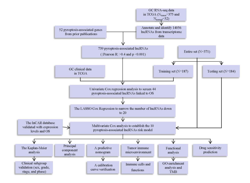
Gastric cancer (GC) ranks fifth in prevalence among carcinomas worldwide. Both pyroptosis and long noncoding RNAs (lncRNAs) play crucial roles in the occurrence and development of gastric cancer. Therefore, we aimed to construct a pyroptosis-associated lncRNA model to predict the outcomes of patients with gastric cancer.
Pyroptosis-associated lncRNAs were identified through co-expression analysis. Univariate and multivariate Cox regression analyses were performed using the least absolute shrinkage and selection operator (LASSO). Prognostic values were tested through principal component analysis, a predictive nomogram, functional analysis and Kaplan‒Meier analysis. Finally, immunotherapy and drug susceptibility predictions and hub lncRNA validation were performed.
Using the risk model, GC individuals were classified into two groups: low-risk and high-risk groups. The prognostic signature could distinguish the different risk groups based on principal component analysis. The area under the curve and the conformance index suggested that this risk model was capable of correctly predicting GC patient outcomes. The predicted incidences of the one-, three-, and five-year overall survivals exhibited perfect conformance. Distinct changes in immunological markers were noted between the two risk groups. Finally, greater levels of appropriate chemotherapies were required in the high-risk group. AC005332.1, AC009812.4 and AP000695.1 levels were significantly increased in gastric tumor tissue compared with normal tissue.
We created a predictive model based on 10 pyroptosis-associated lncRNAs that could accurately predict the outcomes of GC patients and provide a promising treatment option in the future.
Citation: Jinsong Liu, Yuyang Dai, Yueyao Lu, Xiuling Liu, Jianzhong Deng, Wenbin Lu, Qian Liu. Identification and validation of a new pyroptosis-associated lncRNA signature to predict survival outcomes, immunological responses and drug sensitivity in patients with gastric cancer[J]. Mathematical Biosciences and Engineering, 2023, 20(2): 1856-1881. doi: 10.3934/mbe.2023085
Gastric cancer (GC) ranks fifth in prevalence among carcinomas worldwide. Both pyroptosis and long noncoding RNAs (lncRNAs) play crucial roles in the occurrence and development of gastric cancer. Therefore, we aimed to construct a pyroptosis-associated lncRNA model to predict the outcomes of patients with gastric cancer.
Pyroptosis-associated lncRNAs were identified through co-expression analysis. Univariate and multivariate Cox regression analyses were performed using the least absolute shrinkage and selection operator (LASSO). Prognostic values were tested through principal component analysis, a predictive nomogram, functional analysis and Kaplan‒Meier analysis. Finally, immunotherapy and drug susceptibility predictions and hub lncRNA validation were performed.
Using the risk model, GC individuals were classified into two groups: low-risk and high-risk groups. The prognostic signature could distinguish the different risk groups based on principal component analysis. The area under the curve and the conformance index suggested that this risk model was capable of correctly predicting GC patient outcomes. The predicted incidences of the one-, three-, and five-year overall survivals exhibited perfect conformance. Distinct changes in immunological markers were noted between the two risk groups. Finally, greater levels of appropriate chemotherapies were required in the high-risk group. AC005332.1, AC009812.4 and AP000695.1 levels were significantly increased in gastric tumor tissue compared with normal tissue.
We created a predictive model based on 10 pyroptosis-associated lncRNAs that could accurately predict the outcomes of GC patients and provide a promising treatment option in the future.

| [1] |
Y. Shao, H. Jia, S. Li, L. Huang, B. Aikemu, G. Yang, et al., Comprehensive analysis of ferroptosis-related markers for the clinical and biological value in gastric cancer, Oxid. Med. Cell. Longev., 2021 (2021), 7007933. https://doi.org/10.1155/2021/7007933 doi: 10.1155/2021/7007933

|
| [2] |
H. Sung, J. Ferlay, R. L. Siegel, M. Laversanne, I. Soerjomataram, A. Jemal, et al., Global Cancer Statistics 2020: GLOBOCAN estimates of incidence and mortality worldwide for 36 cancers in 185 countries, CA Cancer J. Clin., 71 (2021), 209–249. https://doi.org/10.3322/caac.21660 doi: 10.3322/caac.21660
|
| [3] |
E. C. Smyth, M. Nilsson, H. IGrabsch, N. C. T. van Grieken, F. Lordick, Gastric cancer, Lancet, 396 (2020), 635–648. https://doi.org/10.1016/S0140-6736(20)31288-5 doi: 10.1016/S0140-6736(20)31288-5
|
| [4] |
F. Lordick, K. Shitara, Y. Y. Janjigian, New agents on the horizon in gastric cancer, Ann. Oncol., 28 (2017), 1767–1775. https://doi.org/10.1093/annonc/mdx051 doi: 10.1093/annonc/mdx051
|
| [5] |
Y. Liu, N. S. Sethi, T. Hinoue, B. G. Schneider, A. D. Cherniack, F. Sanchez-Vega, et al., Comparative molecular analysis of gastrointestinal adenocarcinomas, Cancer Cell, 33 (2018), 721–735. https://doi.org/10.1016/j.ccell.2018.03.010 doi: 10.1016/j.ccell.2018.03.010
|
| [6] | The Cancer Genome Atlas Research Network, Comprehensive molecular characterization of gastric adenocarcinoma, Nature, 513 (2014), 202–209. https://doi.org/10.1038%2Fnature13480 |
| [7] |
Y. Tan, Q. Chen, X. Li, Z. Zeng, W. Xiong, G. Li, et al., Pyroptosis: a new paradigm of cell death for fighting against cancer, J. Exp. Clin. Cancer Res., 40 (2021), 153. https://doi.org/10.1186/s13046-021-01959-x doi: 10.1186/s13046-021-01959-x
|
| [8] |
X. Liu, S. Xia, Z. Zhang, H. Wu, J. Lieberman, Channelling inflammation: gasdermins in physiology and disease, Nat. Rev. Drug Discov., 20 (2021), 384–405. https://doi.org/10.1038/s41573-021-00154-z doi: 10.1038/s41573-021-00154-z
|
| [9] |
J. Shi, W. Gao, F. Shao, Pyroptosis: Gasdermin-mediated programmed necrotic cell death, Trends Biochem. Sci., 42 (2017), 245–254. https://doi.org/10.1016/j.tibs.2016.10.004 doi: 10.1016/j.tibs.2016.10.004
|
| [10] |
Z. Zeng, G. Li, S. Wu, Z. Wang, Role of pyroptosis in cardiovascular disease, Cell Prolif., 52 (2019), e12563. https://doi.org/10.1111/cpr.12563 doi: 10.1111/cpr.12563
|
| [11] |
J. Yu, S. Li, J. Qi, Z. Chen, Y. Wu, J. Guo, et al., Cleavage of GSDME by caspase-3 determines lobaplatin-induced pyroptosis in colon cancer cells, Cell Death Dis., 10 (2019), 193. https://doi.org/10.1038/s41419-019-1441-4 doi: 10.1038/s41419-019-1441-4
|
| [12] |
C. Lin, L. Yang, Long noncoding RNA in cancer: Wiring signaling circuitry, Trends Cell Biol., 28 (2018), 287–301. https://doi.org/10.1016/j.tcb.2017.11.008 doi: 10.1016/j.tcb.2017.11.008
|
| [13] |
J. J. Quinn, H. Y. Chang, Unique features of long non-coding RNA biogenesis and function, Nat. Rev. Genet., 17 (2016), 47–62. https://doi.org/10.1038/nrg.2015.10 doi: 10.1038/nrg.2015.10
|
| [14] |
Y. Huang, J. Zhang, L. Hou, G. Wang, H. Liu, R. Zhang, et al., LncRNA AK023391 promotes tumorigenesis and invasion of gastric cancer through activation of the PI3K/Akt signaling pathway, J. Exp. Clin. Cancer Res., 36 (2017), 194. https://doi.org/10.1186/s13046-017-0666-2 doi: 10.1186/s13046-017-0666-2
|
| [15] |
G. Zhang, S. Li, J. Lu, Y. Ge, Q. Wang, G. Ma, et al., LncRNA MT1JP functions as a ceRNA in regulating FBXW7 through competitively binding to miR-92a-3p in gastric cancer, Mol. Cancer, 17 (2018), 87. https://doi.org/10.1186/s12943-018-0829-6 doi: 10.1186/s12943-018-0829-6
|
| [16] |
H. T. Liu, S. Liu, L. Liu, R. R. Ma, P. Gao, EGR1-mediated transcription of lncRNA-HNF1A-AS1 promotes cell-cycle progression in gastric cancer, Cancer Res., 78 (2018), 5877–5890. https://doi.org/10.1158/0008-5472.CAN-18-1011 doi: 10.1158/0008-5472.CAN-18-1011
|
| [17] | M. Arunkumar, C. E. Zielinski, T-Cell receptor repertoire analysis with computational tools-an immunologist's perspective, Cells, 10 (2021), 3582. |
| [18] |
F. Sun, J. Sun, Q. Zhao, A deep learning method for predicting metabolite-disease associations via graph neural network, Briefings Bioinf., 23 (2022), bbac266. https://doi.org/10.1093/bib/bbac266 doi: 10.1093/bib/bbac266
|
| [19] |
R. C. Deo, Machine learning in medicine, Circulation, 132 (2015), 1920–1930. https://doi.org/10.1161/CIRCULATIONAHA.115.001593 doi: 10.1161/CIRCULATIONAHA.115.001593
|
| [20] |
C. Bock, T. Lengauer, Computational epigenetics, Bioinformatics, 24 (2008), 1–10. https://doi.org/10.1093/bioinformatics/btm546 doi: 10.1093/bioinformatics/btm546
|
| [21] |
F. Xu, X. Huang, Y. Li, Y. Chen, L. Lin, m(6)A-related lncRNAs are potential biomarkers for predicting prognoses and immune responses in patients with LUAD, Mol. Ther. Nucleic Acids, 24 (2021), 780–791. https://doi.org/10.1016/j.omtn.2021.04.003 doi: 10.1016/j.omtn.2021.04.003
|
| [22] | D Zheng, L Yu, Z Wei, K Xia, W Guo, N6-methyladenosine-related lncRNAs are potential prognostic biomarkers and correlated with tumor immune microenvironment in osteosarcoma, Front. Genet., 12 (2021), 805607. |
| [23] |
X. Guo, W. Zhong, Y. Chen, W. Zhang, J. Ren, A. Gao, Benzene metabolites trigger pyroptosis and contribute to haematotoxicity via TET2 directly regulating the Aim2/Casp1 pathway, EBioMedicine, 47 (2019), 578–589. https://doi.org/10.1016/j.ebiom.2019.08.056 doi: 10.1016/j.ebiom.2019.08.056
|
| [24] |
F. F. S. Ke, H. K. Vanyai, A. D. Cowan, A. R. D. Delbridge, L. Whitehead, S. Grabow, et al., Embryogenesis and adult life in the absence of intrinsic apoptosis effectors BAX, BAK, and BOK, Cell, 173 (2018), 1217–1230.e17. https://doi.org/10.1016/j.cell.2018.04.036 doi: 10.1016/j.cell.2018.04.036
|
| [25] |
J. Shi, Y. Zhao, K. Wang, X. Shi, Y. Wang, H. Huang, et al., Cleavage of GSDMD by inflammatory caspases determines pyroptotic cell death, Nature, 526 (2015), 660–665. https://doi.org/10.1038/nature15514 doi: 10.1038/nature15514
|
| [26] |
Y. Fang, S. Tian, Y. Pan, W. Li, Q. Wang, Y. Tang, et al., Pyroptosis: A new frontier in cancer, Biomed. Pharmacother., 121 (2020), 109595. https://doi.org/10.1016/j.biopha.2019.109595 doi: 10.1016/j.biopha.2019.109595
|
| [27] | Z. Li, Y. Jia, Y. Feng, R. Cui, R. Miao, X. Zhang, et al., Methane alleviates sepsis-induced injury by inhibiting pyroptosis and apoptosis: In vivo and in vitro experiments, Aging, 11 (2019), 1226–1239. https://doi.org/10.18632%2Faging.101831 |
| [28] |
B. Liu, R. He, L. Zhang, B. Hao, W. Jiang, W. Zhang, et al., Inflammatory caspases drive pyroptosis in acute lung injury, Front. Pharmacol., 12 (2021), 631256. https://doi.org/10.3389/fphar.2021.631256 doi: 10.3389/fphar.2021.631256
|
| [29] |
D. D. Tian, M. Wang, A. Liu, M. R. Gao, C. Qiu, W. Yu, et al., Antidepressant effect of paeoniflorin is through inhibiting pyroptosis CASP-11/GSDMD pathway, Mol. Neurobiol., 58 (2021), 761–776. https://doi.org/10.1007/s12035-020-02144-5 doi: 10.1007/s12035-020-02144-5
|
| [30] |
Y. L. Gao, J. H. Zhai, Y. F. Chai, Recent advances in the molecular mechanisms underlying pyroptosis in sepsis, Mediators Inflamm, 2018 (2018), 5823823. https://doi.org/10.1155/2018/5823823 doi: 10.1155/2018/5823823
|
| [31] |
K. S. Schneider, C. J. Groß , R. F. Dreier, B. S. Saller, R. Mishra, O. Gorka, et al., The inflammasome drives GSDMD-independent secondary pyroptosis and IL-1 release in the absence of Caspase-1 protease activity, Cell Rep., 21 (2017), 3846–3859. https://doi.org/10.1016/j.celrep.2017.12.018 doi: 10.1016/j.celrep.2017.12.018
|
| [32] |
A. Malik, T. D. Kanneganti, Inflammasome activation and assembly at a glance, J. Cell Sci., 130 (2017), 3955–3963. https://doi.org/10.1242/jcs.207365 doi: 10.1242/jcs.207365
|
| [33] |
E. Scosyrev, E. Glimm, Power analysis for multivariable Cox regression models, Stat. Med., 38 (2019), 88–99. https://doi.org/10.1002/sim.7964 doi: 10.1002/sim.7964
|
| [34] |
P. C. Schober, C. Boer, L. A. Schwarte, Correlation coefficients: Appropriate use and interpretation, Anesth. Analg., 126 (2018), 1763–1768. https://doi.org/10.1213/ANE.0000000000002864 doi: 10.1213/ANE.0000000000002864
|
| [35] | S. Xu, D. Liu, T. Chang, X. Wen, S. Ma, G. Sun, et al., Cuproptosis-associated lncRNA establishes new prognostic profile and predicts immunotherapy response in clear cell renal cell carcinoma, Front. Genet., 13 (2022), 938259. https://doi.org/10.3389%2Ffgene.2022.938259 |
| [36] | X. Ma, C. Mo, L. Huang, P. Cao, L. Shen, C. Gui, An robust rank aggregation and least absolute shrinkage and selection operator analysis of novel gene signatures in dilated cardiomyopathy, Front. Cardiovasc. Med., 8 (2021), 747803. https://doi.org/10.3389%2Ffcvm.2021.747803 |
| [37] |
X. Liu, D. Wang, S. Han, F. Wang, Z. Zang, C. Xu, et al., Signature of m5C-Related lncRNA for prognostic prediction and immune responses in pancreatic cancer, J. Oncol., 2022 (2022), 7467797. https://doi.org/10.1155/2022/7467797 doi: 10.1155/2022/7467797
|
| [38] |
Y. Li, J. Wang, F. Wang, C. Gao, Y. Cao, J. Wang, et al., Development and verification of an autophagy-related lncRNA signature to predict clinical outcomes and therapeutic responses in ovarian cancer, Front. Med., 8 (2021), 715250. https://doi.org/10.3389/fmed.2021.715250 doi: 10.3389/fmed.2021.715250
|
| [39] |
J. X. Mi, Y. N. Zhang, Z. Lai, W. Li, L. Zhou, F. Zhong, Principal component analysis based on nuclear norm minimization, Neural Networks, 118 (2019), 1–16. https://doi.org/10.1016/j.neunet.2019.05.020 doi: 10.1016/j.neunet.2019.05.020
|
| [40] |
S. Lacny, T. Wilson, F. Clement, D. J. Roberts, P. Faris, W. A. Ghali, et al., Kaplan-Meier survival analysis overestimates cumulative incidence of health-related events in competing risk settings: a meta-analysis, J. Clin. Epidemiol., 93 (2018), 25–35. https://doi.org/10.1016/j.jclinepi.2017.10.006 doi: 10.1016/j.jclinepi.2017.10.006
|
| [41] |
J. Y. Ma, S. Liu, J. Chen, Q. Liu, Metabolism-related long non-coding RNAs (lncRNAs) as potential biomarkers for predicting risk of recurrence in breast cancer patients, Bioengineered, 12 (2021), 3726–3736. https://doi.org/10.1080/21655979.2021.1953216 doi: 10.1080/21655979.2021.1953216
|
| [42] | Y. Wang, J. Li, Y. Xia, R. Gong, K. Wang, Z. Yan, et al., Prognostic nomogram for intrahepatic cholangiocarcinoma after partial hepatectomy, J. Clin. Oncol., 31 (2013), 1188–1195. |
| [43] |
W. Lv, Y. Tan, C. Zhao, Y. Wang, M. Wu, Y. Wu, et al., Identification of pyroptosis-related lncRNAs for constructing a prognostic model and their correlation with immune infiltration in breast cancer, J. Cell. Mol. Med., 25 (2021), 10403–10417. https://doi.org/10.1111/jcmm.16969 doi: 10.1111/jcmm.16969
|
| [44] |
M. Li, W. Cao, B. Huang, Z. Zhu, Y. Chen, J. Zhang, et al., Establishment and analysis of an individualized immune-related gene signature for the prognosis of gastric cancer, Front. Surg., 9 (2022), 829237. https://doi.org/10.3389/fsurg.2022.829237 doi: 10.3389/fsurg.2022.829237
|
| [45] |
Y. Chen, C. Zhang, X. Zou, M. Yu, B. Yang, C. F. Ji, et al., Identification of macrophage related gene in colorectal cancer patients and their functional roles, BMC Med. Genomics, 14 (2021), 159. https://doi.org/10.1186/s12920-021-01010-0 doi: 10.1186/s12920-021-01010-0
|
| [46] |
W. Yang, J. Soares, P. Greninger, E. J. Edelman, H. Lightfoot, S. Forbes, et al., Genomics of drug sensitivity in cancer (GDSC): A resource for therapeutic biomarker discovery in cancer cells, Nucleic Acids Res., 41 (2013), 955–961. https://doi.org/10.1093/nar/gks1111 doi: 10.1093/nar/gks1111
|
| [47] |
Y. Zheng, Q. Xu, M. Liu, H. Hu, Y. Xie, Z. Zuo, et al., lnCAR: A comprehensive resource for lncRNAs from cancer arrays, Cancer Res., 79 (2019), 2076–2083. https://doi.org/10.1158/0008-5472.CAN-18-2169 doi: 10.1158/0008-5472.CAN-18-2169
|
| [48] |
T. Han, D. Xu, J. Zhu, J. Li, L. Liu, Y. Deng, Identification of a robust signature for clinical outcomes and immunotherapy response in gastric cancer: Based on N6-methyladenosine related long noncoding RNAs, Cancer Cell Int., 21 (2021), 432. https://doi.org/10.1186/s12935-021-02146-w doi: 10.1186/s12935-021-02146-w
|
| [49] | S. Kesavardhana, R. K. S. Malireddi, T. D. Kanneganti, Caspases in cell death, inflammation, and gasdermin-induced pyroptosis, Annu. Rev. Immunol., 38 (2020), 567–595. https://doi.org/10.1146%2Fannurev-immunol-073119-095439 |
| [50] | X. Ma, P. Guo, Y. Qiu, K. Mu, L. Zhu, W. Zhao, et al., Loss of AIM2 expression promotes hepatocarcinoma progression through activation of mTOR-S6K1 pathway, Oncotarget, 7 (2016), 36185–36197. https://doi.org/10.18632%2Foncotarget.9154 |
| [51] | F. Su, J. Duan, J. Zhu, H. Fu, X. Zheng, C. Ge, Long noncoding RNA nuclear paraspeckle assembly transcript 1 regulates ionizing radiationinduced pyroptosis via microRNA448/gasdermin E in colorectal cancer cells, Int. J. Oncol., 59 (2021), 1–11. https://doi.org/10.3892%2Fijo.2021.5259 |
| [52] |
L. Jiang, W. Ge, Y. Cui, Z. Wang, The regulation of long non-coding RNA 00958 (LINC00958) for oral squamous cell carcinoma (OSCC) cells death through absent in melanoma 2 (AIM2) depending on microRNA-4306 and Sirtuin1 (SIRT1) in vitro, Bioengineered, 12 (2021), 5085–5098. https://doi.org/10.1080/21655979.2021.1955561 doi: 10.1080/21655979.2021.1955561
|
| [53] |
W. Zhang, Y. Wu, B. Hou, Y. Wang, D. Deng, Z. Fu, et al., A SOX9-AS1/miR-5590-3p/SOX9 positive feedback loop drives tumor growth and metastasis in hepatocellular carcinoma through the Wnt/beta-catenin pathway, Mol. Oncol., 13 (2019), 2194–2210. https://doi.org/10.1002/1878-0261.12560 doi: 10.1002/1878-0261.12560
|
| [54] |
C. Wang, C. D. Han, Q. Zhao, X. Chen, Circular RNAs and complex diseases: from experimental results to computational models, Brief. Bioinf., 22 (2021), bbab286. https://doi.org/10.1093/bib/bbab286 doi: 10.1093/bib/bbab286
|
| [55] |
Y. Wang, X. Huang, S. Chen, H. Jiang, H. Rao, L. Lu, et al., In Silico identification and validation of cuproptosis-related lncRNA signature as a novel prognostic model and immune function analysis in colon adenocarcinoma, Curr. Oncol., 29 (2022), 6573–6593. https://doi.org/10.3390/curroncol29090517 doi: 10.3390/curroncol29090517
|
| [56] |
L. Zhang, T. Liu, H. Chen, Q. Zhao, H. Liu, Predicting lncRNA-miRNA interactions based on interactome network and graphlet interaction, Genomics, 113 (2021), 874–880. https://doi.org/10.1016/j.ygeno.2021.02.002 doi: 10.1016/j.ygeno.2021.02.002
|
| [57] |
L. Zhang, P. Yang, H. Feng, Q. Zhao, H. Liu, Using network distance analysis to predict lncRNA-miRNA interactions, Interdiscip. Sci., 13 (2021), 535–545. https://doi.org/10.1007/s12539-021-00458-z doi: 10.1007/s12539-021-00458-z
|
| [58] |
K. J. Chu, Y. S. Ma, X. H. Jiang, T. M. Wu, Z. J. Wu, Z. Z. Li, et al., Whole-transcriptome sequencing identifies key differentially expressed mRNAs, miRNAs, lncRNAs, and circRNAs associated with CHOL, Mol. Ther. Nucleic Acids, 21 (2020), 592–603. https://doi.org/10.1016/j.omtn.2020.06.025 doi: 10.1016/j.omtn.2020.06.025
|
| [59] |
L. Moreno-García, T. López-Royo, A. C. Calvo, J. M. Toivonen, M. de la Torre, L. Moreno-Martínez, et al., Competing endogenous RNA networks as biomarkers in neurodegenerative diseases, Int. J. Mol. Sci., 21 (2020), 9582. https://doi.org/10.3390/ijms21249582 doi: 10.3390/ijms21249582
|
 mbe-20-02-085 Supplementary Table 1.xlsx mbe-20-02-085 Supplementary Table 1.xlsx |
 |
| mbe-20-02-085 Supplementary Table 2.xlsx |
|


Figures(12)

Jinsong Liu, Yuyang Dai, Yueyao Lu, Xiuling Liu, Jianzhong Deng, Wenbin Lu, Qian Liu. Identification and validation of a new pyroptosis-associated lncRNA signature to predict survival outcomes, immunological responses and drug sensitivity in patients with gastric cancer[J]. Mathematical Biosciences and Engineering, 2023, 20(2): 1856-1881. doi: 10.3934/mbe.2023085


 DownLoad: