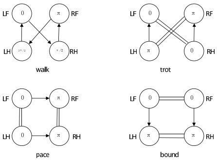
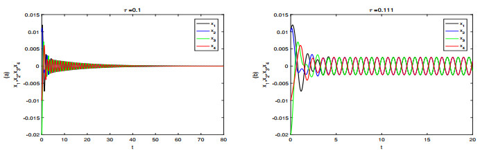
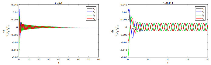
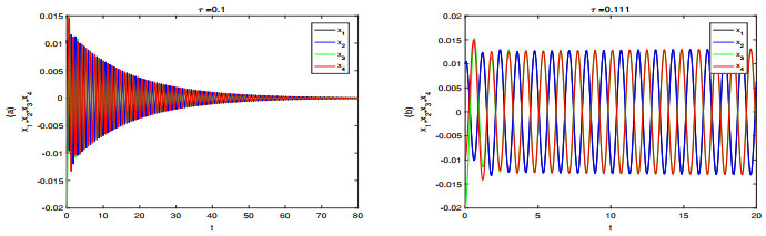
In this paper, Van Der Pol (VDP) oscillators are used as the output signal of central pattern generator (CPG), and a VDP-CPG network system of quadruped with four primary gaits (walk, trot, pace and bound) is established. The existence conditions of Hopf bifurcations for VDP-CPG systems corresponding to four primary gaits are given, and the coupling strength ranges between oscillators for four gaits are obtained. Numerical simulations are used to support theoretical analysis.
Citation: Liqin Liu, Chunrui Zhang. Dynamic properties of VDP-CPG model in rhythmic movement with delay[J]. Mathematical Biosciences and Engineering, 2020, 17(4): 3190-3202. doi: 10.3934/mbe.2020181
In this paper, Van Der Pol (VDP) oscillators are used as the output signal of central pattern generator (CPG), and a VDP-CPG network system of quadruped with four primary gaits (walk, trot, pace and bound) is established. The existence conditions of Hopf bifurcations for VDP-CPG systems corresponding to four primary gaits are given, and the coupling strength ranges between oscillators for four gaits are obtained. Numerical simulations are used to support theoretical analysis.

| [1] |
M. Land, Eye movements in man and other animals, Vision Res., 162 (2019), 1-7. doi: 10.1016/j.visres.2019.06.004

|
| [2] |
M. Manookin, S. Patterson, C. Linehan, Neural mechanisms mediating motion sensitivity in parasol ganglion cells of the primate retina, Neuron, 97 (2018), 1327-1340.e4. doi: 10.1016/j.neuron.2018.02.006
|
| [3] |
M. Creamer, O. Mano, D. A. Clark, Visual control of walking speed in drosophila, Neuron 100 (2018), 1460-1473.e6. doi: 10.1016/j.neuron.2018.10.028
|
| [4] |
T. Marques, M. T. Summers, G. Fioreze, M. Fridman, R. F. Dias, M. B. Feller, et al., A role for mouse primary visual cortex in motion perception, Curr. Biol., 28 (2018), 1703-1713.e6. doi: 10.1016/j.cub.2018.04.012
|
| [5] |
F. Delcomyn, Neural basis of rhythmic behavior in animals, Science, 210 (1980), 492-498. doi: 10.1126/science.7423199
|
| [6] | K. Sigvardt, T. Williams, Models of central pattern generators as oscillators: the lamprey locomotor CPG, in Seminars in Neuroscience, Academic Press, (1992), 37-46. |
| [7] | S. Hooper, Central pattern generators, Current Biology, 10 (2000), 176-179. |
| [8] | T. Yamaguchi, The central pattern generator for forelimb locomotion in the cat, in Progress in Brain Research, Elsevier, (2004), 115-122. |
| [9] |
C. Bal, G. O. Koca, D. Korkmaz, Z. H. Akpolat, M. Ay, CPG-based autonomous swimming control for multi-tasks of a biomimetic robotic fish, Ocean Eng., 189 (2019), 106334. doi: 10.1016/j.oceaneng.2019.106334
|
| [10] |
D. Tran, L. Koo, Y. Lee, H. Moon, S. Parket, J. C. Koo, et al., Central pattern generator based reflexive control of quadruped walking robots using a recurrent neural network, Rob. Auton. Sys., 62 (2014), 1497-1516. doi: 10.1016/j.robot.2014.05.011
|
| [11] |
J. Zhang, F. Gao, X. Han, X. Chen, X. Han, Trot gait design and CPG method for a quadruped robot, J. Bionic. Eng., 11 (2014), 18-25. doi: 10.1016/S1672-6529(14)60016-0
|
| [12] | H. Xu, J. Gan, J. Ren, B. R. Wang, Y. L. Jin, Gait CPG adjustment for a quadruped robot based on Hopf oscillator, J. Syst. Simul., 29 (2017), 3092-3099. |
| [13] | H. Liu, W. Jia, L. Bi, Hopf oscillator based adaptive locomotion control for a bionic quadruped robot, 2017 IEEE International Conference on Mechatronics and Automation, 2017. Available from: https://ieeexplore.ieee.org/abstract/document/8015944/. |
| [14] | C. Liu, Q. Chen, J. Zhang, Coupled Van der Pol oscillators utilised as central pattern generators for quadruped locomotion, 2009 Chinese Control and Decision Conference, 2009. Available from: https://ieeexplore.ieee.org/abstract/document/5192385. |
| [15] |
S. Dixit, A. Sharma, M. Shrimali, The dynamics of two coupled Van der Pol oscillators with attractive and repulsive coupling, Phys. Lett. A, 383 (2019), 125930. doi: 10.1016/j.physleta.2019.125930
|
| [16] |
J. Collins, I. Stewart, Coupled nonlinear oscillators and the symmetries of animal gaits, J. Nonlinear Sci., 3 (1993), 349-392. doi: 10.1007/BF02429870
|
| [17] |
P. L. Buono, M. Golubitsky, Models of central pattern generators for quadruped locomotion Ⅰ. Primary gaits, J. Math. Biol., 42 (2001), 291-326. doi: 10.1007/s002850000058
|
| [18] |
P. L. Buono, Models of central pattern generators for quadruped locomotion Ⅱ. Secondary gaits, J. Math. Biol., 42 (2001), 327-346. doi: 10.1007/s002850000073
|
| [19] | Y. Song, J. Xu, T. Zhang, Bifurcation, amplitude death and oscillation patterns in a system of three coupled van der Pol oscillators with diffusively delayed velocity coupling, CHA, 21 (2011), 023111. |
| [20] | C. Zhang, B. Zheng, L. Wang, Multiple Hopf bifurcation of three coupled van der Pol oscillators with delay, Appl. Math. Comput., 217 (2011), 7155-7166. |
Figures(4)

Liqin Liu, Chunrui Zhang. Dynamic properties of VDP-CPG model in rhythmic movement with delay[J]. Mathematical Biosciences and Engineering, 2020, 17(4): 3190-3202. doi: 10.3934/mbe.2020181


 DownLoad: