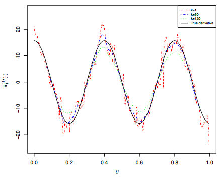
In varying-coefficient models, accurately estimating the derivatives of coefficient functions is crucial, particularly for optimal bandwidth selection and confidence interval construction. Despite its importance, methods have largely ignored derivative estimation. In this paper, we addresse this gap by proposing a novel weighted difference quotient approach to estimate both first and second order derivatives of coefficient functions under the differences in the smoothness of the coefficient functions. We derived the asymptotic properties of our estimator and introduced a data-driven tuning parameter selection method. Simulations and real-data analyses confirmed the superior performance of our approach compared to existing techniques. Our method provides the most accurate estimates, effectively estimating both the first and second derivatives.
Citation: Junfeng Huo, Mingquan Wang, Xiuqing Zhou. Nonparametric estimation of coefficient function derivatives in varying coefficient models[J]. AIMS Mathematics, 2025, 10(5): 11592-11626. doi: 10.3934/math.2025526
In varying-coefficient models, accurately estimating the derivatives of coefficient functions is crucial, particularly for optimal bandwidth selection and confidence interval construction. Despite its importance, methods have largely ignored derivative estimation. In this paper, we addresse this gap by proposing a novel weighted difference quotient approach to estimate both first and second order derivatives of coefficient functions under the differences in the smoothness of the coefficient functions. We derived the asymptotic properties of our estimator and introduced a data-driven tuning parameter selection method. Simulations and real-data analyses confirmed the superior performance of our approach compared to existing techniques. Our method provides the most accurate estimates, effectively estimating both the first and second derivatives.

| [1] | B. R. H. Shumway, Applied Statistical Time Series Analysis, New Jersey: Prentice Hall, 1988. http://dx.doi.org/10.1007/978-1-4757-3261-0 |
| [2] |
T. J. Hastie, R. J. Tibshirani, Varying-coefficient models, J. Roy. Statist. Soc. Ser. B, 4 (1993), 757–796. https://doi.org/10.1111/j.2517-6161.1993.tb01939.x doi: 10.1111/j.2517-6161.1993.tb01939.x

|
| [3] |
J. Fan, W. Zhang, Statistical estimation in varying coefficient models, Ann. Statist., 27 (1999), 1491–1518. https://doi.org/10.1214/aos/1017939139 doi: 10.1214/aos/1017939139
|
| [4] |
J. Z. Huang, H. Shen, Functional coefficient regression models for non-linear time series: A polynomial spline approach, Scand. J. Statist., 31 (2004), 515–534. https://doi.org/10.1111/j.1467-9469.2004.00404.x doi: 10.1111/j.1467-9469.2004.00404.x
|
| [5] |
Z. Cai, J. Fan, R. Li, Efficient estimation and inferences for varying-coefficient models, J. Amer. Statist. Assoc., 95 (2000), 888–902. https://doi.org/10.1080/01621459.2000.10474280 doi: 10.1080/01621459.2000.10474280
|
| [6] | T. V. Somanathan, V. A. Nageswaran, The economics of derivatives, Cambridge University Press, London, 2015. https://doi.org/10.1017/CBO9781316134566 |
| [7] |
J. Fan, W. Zhang, Statistical methods with varying coefficient models, Stat. Interface, 2008 (2008), 179–195. https://doi.org/10.4310/SII.2008.v1.n1.a15 doi: 10.4310/SII.2008.v1.n1.a15
|
| [8] |
C. T. Chiang, J. A. Rice, C. O. Wu, Smoothing spline estimation for varying coefficient models with repeatedly measured dependent variables, J. Amer. Statist. Assoc., 96 (2001), 605–619. https://doi.org/10.1198/016214501753168280 doi: 10.1198/016214501753168280
|
| [9] |
W. S. Cleveland, S. J. Devlin, Locally weighted regression: an approach to regression analysis by local fitting, J. Amer. Statist. Assoc., 83 (1988), 596–610. https://doi.org/10.1080/01621459.1988.10478639 doi: 10.1080/01621459.1988.10478639
|
| [10] | J. Fan, I. Gijbels, A Local polynomial modelling and its applications, Chapman & Hall, London, 1996. https://doi.org/10.1201/9780203748725 |
| [11] | P. J. Green, B. W. Silverman, Nonparametric regression and generalized linear models, Chapman & Hall, London, 1994. http://dx.doi.org/10.1007/978-1-4899-4473-3 |
| [12] |
H. Wang, X. Zhou, Explicit estimation of derivatives from data and differential equations by Gaussian process regression, Int. J. Uncertain. Quantif., 11 (2021), 41–57. https://doi.org/10.1615/Int.J.UncertaintyQuantification.2021034382 doi: 10.1615/Int.J.UncertaintyQuantification.2021034382
|
| [13] |
Z. Liu, M. Li, On the estimation of derivatives using plug-in kernel ridge regression estimators, J. Mach. Learn. Res., 24 (2023), 1–37. https://doi.org/10.1007/s00180-007-0102-8 doi: 10.1007/s00180-007-0102-8
|
| [14] |
H. G. Müller, U. Stadtmüller, T. Schmitt, Bandwidth choice and confidence intervals for derivatives of noisy data, Biometrika, 74 (1987), 743–749. https://doi.org/10.1093/biomet/74.4.743 doi: 10.1093/biomet/74.4.743
|
| [15] |
R. Charnigo, B. Hall, C. Srinivasan, A generalized Cp criterion for derivative estimation, Technometrics, 53 (2011), 238–253. https://doi.org/10.1198/TECH.2011.09147 doi: 10.1198/TECH.2011.09147
|
| [16] |
K. D. Brabanter, J. D. Brabanter, B. D. Moor, I. Gijbels, Derivative estimation with local polynomial fitting, J. Mach. Learn. Res., 14 (2013), 281–301. https://doi.org/10.1002/cem.2489 doi: 10.1002/cem.2489
|
| [17] |
W. Wang, L. Lin, Derivative estimation based on difference sequence via locally weighted least squares regression, J. Mach. Learn. Res., 16 (2015), 2617–2641. https://doi.org/10.5555/2789272.2912083 doi: 10.5555/2789272.2912083
|
| [18] |
W. Dai, T. Tong, M. G. Genton, Optimal estimation of derivatives in nonparametric regression, J. Mach. Learn. Res., 17 (2016), 1–37. https://doi.org/10.5555/2946645.3053446 doi: 10.5555/2946645.3053446
|
| [19] |
Y. Liu, K. D. Brabanter, Smoothed nonparametric derivative estimation using weighted difference quotients, J. Mach. Learn. Res., 21 (2020), 1–45. https://doi.org/10.5555/3455716.3455781 doi: 10.5555/3455716.3455781
|
| [20] |
S. Liu, X. Kong, A generalized correlated $C_ p$ criterion for derivative estimation with dependent errors, Comput. Statist. Data Anal., 21 (2022), 1–23. https://doi.org/10.1016/j.csda.2022.107473 doi: 10.1016/j.csda.2022.107473
|
| [21] |
J. Huo, X. Zhou, Efficient estimation in varying coefficient regression models, J. Stat. Comput. Simul., 93 (2023), 2297–2320. https://doi.org/10.1080/00949655.2023.2179626 doi: 10.1080/00949655.2023.2179626
|
| [22] |
H. Wang, Y. Xia, Shrinkage estimation of the varying coefficient model, J. Amer. Statist. Assoc., 104 (2009), 747–757. https://doi.org/10.1198/jasa.2009.0138 doi: 10.1198/jasa.2009.0138
|
| [23] |
Y. Zhao, J. Lin, X. Huang, H. Wang, Adaptive jump-preserving estimates in varying-coefficient models, J. Multivariate Anal., 149 (2016), 65–80. https://doi.org/10.1016/j.jmva.2016.03.005 doi: 10.1016/j.jmva.2016.03.005
|
| [24] |
E. Parzen, On estimation of a probability density function and mode, Ann. Math. Statist., 33 (1962), 1065–1076. https://doi.org/10.1214/aoms/1177704472 doi: 10.1214/aoms/1177704472
|
| [25] |
J. Ormerod, M. P. Wand, I. Koch, Penalised spline support vector classifiers: computational issues, Comput. Statist., 23 (2008), 623–641. https://doi.org/10.1007/s00180-007-0102-8 doi: 10.1007/s00180-007-0102-8
|
| [26] | S. Kotz, N. Balakrishnan, C. B. Read, B. Vidakovic, N. L. Johnson, Encyclopedia of Statistical Sciences, Volume 1. John Wiley & Sons, 2005. https://doi.org/110.1002/0471667196 |
| [27] |
J. Fan, T. Huang, Profile likelihood inferences on semiparametric varying-coefficient partially linear models, Bernoulli, 11 (2005), 1031–1057. https://doi.org/10.3150/bj/1137421639 doi: 10.3150/bj/1137421639
|
| [28] |
Y. P. Mack, B. W. Silverman, Weak and strong uniform consistency of kernel regression estimates, Z. Wahrsch. Verw. Gebiete, 61 (1982), 405–415. https://doi.org/10.1007/BF00539840 doi: 10.1007/BF00539840
|
| [29] |
K. F. Cheng, R. L. Taylor, On the uniform complete convergence of estimates for multivariate density functions and regression curves, Ann. Inst. Statist. Math., 32 (1980), 187–199. https://doi.org/10.1007/BF00539840 doi: 10.1007/BF00539840
|
| [30] | H. A. David, H. W. Nagaraja, Order Statistics, 3 Eds., John Wiley and Sons Inc, 2005. http://dx.doi.org/10.1002/9781118445112.stat00830 |


Figures(7) / Tables(8)

Junfeng Huo, Mingquan Wang, Xiuqing Zhou. Nonparametric estimation of coefficient function derivatives in varying coefficient models[J]. AIMS Mathematics, 2025, 10(5): 11592-11626. doi: 10.3934/math.2025526


 DownLoad: