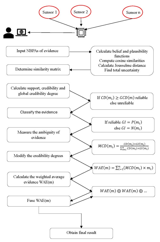
The Dempster–Shafer evidence theory is a very practical concept for handling uncertain information. The foundation of this theory lies in the basic probability assignment (BPA), which exclusively accounts for the degree of support attributed to focal elements (FEs). In this study, neutrosophic evidence sets (NESs) are defined to introduce additional probabilistic measures, aimed at addressing the uncertainty, imprecision, incompleteness, and inconsistency present in real-world information. The basic element of NESs is a neutrosophic basic probability assignment (NBPA), which consists of three components. The truth degree of FEs is represented by the first BPA, the second BPA represents the indeterminacy degree of FEs, and the last BPA characterizes the falsity degree of FEs. In NESs, each support degree of FEs is shown separately without any limitation. Therefore, the general concept of NESs is broader compared to traditional evidence sets and intuitionistic fuzzy evidence sets. Unlike the neutrosophic set (NS), the NBPA method assigns truth-support, uncertainty-support, and false-support degrees, as well as these support degrees, to single and multiple subsets in a discriminative framework. This paper aimed to develop some information measures for NESs, such as neutrosophic Deng entropy (NDE), neutrosophic cosine similarity measure, and neutrosophic Jousselme distance. Then, an improved method based on NDE and neutrosophic cosine similarity measure was established to combine contradictory evidence to increase the influence of reliable evidence on the one hand and to reduce the influence of unreliable evidence on the other hand. Finally, a case involving sensor data integration for target identification was studied to highlight the importance of these innovative ideas. The numerical example demonstrates that the proposed method provides more reliable and superior fusion performance compared to classical models, particularly in scenarios involving high conflict and uncertain information. However, the effectiveness of the method is partially influenced by the structure of the similarity matrix and the entropy parameters, which necessitates careful parameter tuning to achieve optimal results. These limitations are explicitly highlighted to serve as a guide for future improvements and broader applications of the method.
Citation: Ali Köseoğlu, Rıdvan Şahin, Ümit Demir. Multi-sensor data fusion based on the similarity measure and belief (Deng) entropy under neutrosophic evidence sets[J]. AIMS Mathematics, 2025, 10(5): 10471-10503. doi: 10.3934/math.2025477
The Dempster–Shafer evidence theory is a very practical concept for handling uncertain information. The foundation of this theory lies in the basic probability assignment (BPA), which exclusively accounts for the degree of support attributed to focal elements (FEs). In this study, neutrosophic evidence sets (NESs) are defined to introduce additional probabilistic measures, aimed at addressing the uncertainty, imprecision, incompleteness, and inconsistency present in real-world information. The basic element of NESs is a neutrosophic basic probability assignment (NBPA), which consists of three components. The truth degree of FEs is represented by the first BPA, the second BPA represents the indeterminacy degree of FEs, and the last BPA characterizes the falsity degree of FEs. In NESs, each support degree of FEs is shown separately without any limitation. Therefore, the general concept of NESs is broader compared to traditional evidence sets and intuitionistic fuzzy evidence sets. Unlike the neutrosophic set (NS), the NBPA method assigns truth-support, uncertainty-support, and false-support degrees, as well as these support degrees, to single and multiple subsets in a discriminative framework. This paper aimed to develop some information measures for NESs, such as neutrosophic Deng entropy (NDE), neutrosophic cosine similarity measure, and neutrosophic Jousselme distance. Then, an improved method based on NDE and neutrosophic cosine similarity measure was established to combine contradictory evidence to increase the influence of reliable evidence on the one hand and to reduce the influence of unreliable evidence on the other hand. Finally, a case involving sensor data integration for target identification was studied to highlight the importance of these innovative ideas. The numerical example demonstrates that the proposed method provides more reliable and superior fusion performance compared to classical models, particularly in scenarios involving high conflict and uncertain information. However, the effectiveness of the method is partially influenced by the structure of the similarity matrix and the entropy parameters, which necessitates careful parameter tuning to achieve optimal results. These limitations are explicitly highlighted to serve as a guide for future improvements and broader applications of the method.

| [1] |
Y. Jin, J. Branke, Evolutionary optimization in uncertain environments-a survey, IEEE Trans. Evol. Comput., 9 (2005), 303–317. https://doi.org/10.1109/TEVC.2005.846356 doi: 10.1109/TEVC.2005.846356

|
| [2] |
R. R. Yager, Decision making under measure-based granular uncertainty, Granular Comput., 3 (2018), 345–353. https://doi.org/10.1007/S41066-017-0075-0/METRICS doi: 10.1007/S41066-017-0075-0/METRICS
|
| [3] |
L. A. Zadeh, Fuzzy sets, Inf. Control, 8 (1965), 338–353. https://doi.org/10.1016/S0019-9958(65)90241-X doi: 10.1016/S0019-9958(65)90241-X
|
| [4] |
K. T. Atanassov, Intuitionistic fuzzy sets, Fuzzy Sets Syst., 20 (1986), 87–96. https://doi.org/10.1016/S0165-0114(86)80034-3 doi: 10.1016/S0165-0114(86)80034-3
|
| [5] | F. A. Smarandache, Unifying field in logics: neutrosophic logic, American Research Press, 1999. |
| [6] | A. P. Dempster, Upper and lower probabilities induced by a multivalued mapping, In: R. R. Yager, L. Liu, Classic works of the Dempster–Shafer theory of belief functions, 2008, 57–72. https://doi.org/10.1007/978-3-540-44792-4_3 |
| [7] | G. Shafer, A mathematical theory of evidence, Princeton University Press, 1976. https://doi.org/10.1515/9780691214696 |
| [8] | Y. Deng, D numbers: theory and applications, J. Inf. Comput. Sci., 9 (2012), 2421–2428. |
| [9] | H. Wang, F. Smarandache, Y. Q. Zhang, R. Sunderraman, Single valued neutrosophic sets, Multispace Multistructure, 4 (2010), 410–413. |
| [10] |
A. Köseoğlu, R. Şahin, M. Merdan, A simplified neutrosophic multiplicative set-based TODIM using water-filling algorithm for the determination of weights, Expert Syst., 37 (2020) e12515. https://doi.org/10.1111/exsy.12515 doi: 10.1111/exsy.12515
|
| [11] |
A. Köseoğlu, F. Altun, R. Şahin, Aggregation operators of complex fuzzy Z-number sets and their applications in multi-criteria decision making, Complex Intell. Syst., 10 (2024), 6559–6579, https://doi.org/10.1007/S40747-024-01450-y doi: 10.1007/S40747-024-01450-y
|
| [12] |
R. Şahin, M. Yigider, A multi-criteria neutrosophic group decision making method based TOPSIS for supplier selection, Appl. Math. Inf. Sci., 10 (2016), 1843–1852. https://doi.org/10.18576/AMIS/100525 doi: 10.18576/AMIS/100525
|
| [13] | A. Köseoğlu, Generalized correlation coefficients of intuitionistic multiplicative sets and their applications to pattern recognition and clustering analysis, J. Exp. Theor. Artif. Intell., 2024. https://doi.org/10.1080/0952813X.2024.2323039 |
| [14] |
H. Garg, A new exponential-logarithm-based single-valued neutrosophic set and their applications, Expert. Syst. Appl., 238 (2024), 121854. https://doi.org/10.1016/J.ESWA.2023.121854 doi: 10.1016/J.ESWA.2023.121854
|
| [15] |
J. B. Yang, D. L. Xu, Evidential reasoning rule for evidence combination, Artif. Intell., 205 (2013), 1–29. https://doi.org/10.1016/J.ARTINT.2013.09.003 doi: 10.1016/J.ARTINT.2013.09.003
|
| [16] |
C. Fu, J. B. Yang, S. L. Yang, A group evidential reasoning approach based on expert reliability. Eur. J. Oper. Res., 246 (2015), 886–893. https://doi.org/10.1016/J.EJOR.2015.05.042 doi: 10.1016/J.EJOR.2015.05.042
|
| [17] |
V. N. Huynh, T. T. Nguyen, C. A. Le, Adaptively entropy-based weighting classifiers in combination using Dempster–Shafer theory for word sense disambiguation, Comput. Speech Lang, 24 (2010), 461–473. https://doi.org/10.1016/J.CSL.2009.06.003 doi: 10.1016/J.CSL.2009.06.003
|
| [18] |
O. Kharazmi, J. E. Contreras-Reyes, Deng-Fisher information measure and its extensions: application to Conway's game of life, Chaos Solitons Fract., 174 (2023), 113871. https://doi.org/10.1016/J.CHAOS.2023.113871 doi: 10.1016/J.CHAOS.2023.113871
|
| [19] |
O. Kharazmi, J. E. Contreras-Reyes, Belief inaccuracy information measures and their extensions, Fluctuation Noise Lett., 23 (2024), 2450041. https://doi.org/10.1142/S021947752450041X doi: 10.1142/S021947752450041X
|
| [20] |
R. R. Yager, On the Dempster–Shafer framework and new combination rules, Inf. Sci., 41 (1987) 93–137. https://doi.org/10.1016/0020-0255(87)90007-7 doi: 10.1016/0020-0255(87)90007-7
|
| [21] |
D. Dubois, H. Prade, Representation and combination of uncertainty with belief functions and possibility measures, Comput. Intell., 4 (1988), 244–264. https://doi.org/10.1111/J.1467-8640.1988.TB00279.X doi: 10.1111/J.1467-8640.1988.TB00279.X
|
| [22] |
P. Smets, The combination of evidence in the transferable belief model, IEEE Trans. Pattern Anal. Mach. Intell., 12 (1990), 447–458. https://doi.org/10.1109/34.55104 doi: 10.1109/34.55104
|
| [23] |
M. Urbani, G. Gasparini, M. Brunelli, A numerical comparative study of uncertainty measures in the Dempster–Shafer evidence theory, Inf. Sci., 639 (2023), 119027. https://doi.org/10.1016/J.INS.2023.119027 doi: 10.1016/J.INS.2023.119027
|
| [24] |
Q. Zhang, P. Zhang, T. Li, Information fusion for large-scale multi-source data based on the Dempster–Shafer evidence theory, Inf. Fusion, 115 (2025), 102754. https://doi.org/10.1016/J.INFFUS.2024.102754 doi: 10.1016/J.INFFUS.2024.102754
|
| [25] |
M. Brunelli, R. P. Jayasuriya Kuranage, V. N. Huynh, Selection rules for new focal elements in the Dempster–Shafer evidence theory, Inf. Sci., 712 (2025), 122160. https://doi.org/10.1016/J.INS.2025.122160 doi: 10.1016/J.INS.2025.122160
|
| [26] |
Y. Song, X. Wang, J. Zhu, L. Lei, Sensor dynamic reliability evaluation based on evidence theory and intuitionistic fuzzy sets, Appl. Intell., 48 (2018), 3950–3962. https://doi.org/10.1007/S10489-018-1188-0/TABLES/6 doi: 10.1007/S10489-018-1188-0/TABLES/6
|
| [27] |
Y. Song, X. Wang, L. Lei, A. Xue, Combination of interval-valued belief structures based on intuitionistic fuzzy set, Knowl. Based Syst., 67 (2014), 61–70. https://doi.org/10.1016/J.KNOSYS.2014.06.008 doi: 10.1016/J.KNOSYS.2014.06.008
|
| [28] |
Y. Li, Y. Deng, Intuitionistic evidence sets, IEEE Access, 7 (2019), 106417–106426. https://doi.org/10.1109/ACCESS.2019.2932763 doi: 10.1109/ACCESS.2019.2932763
|
| [29] |
Y. Xue, Y. Deng, On the conjunction of possibility measures under intuitionistic evidence sets, J. Ambient Intell. Humanized Comput., 12 (2021), 7827–7836. https://doi.org/10.1007/S12652-020-02508-8/METRICS doi: 10.1007/S12652-020-02508-8/METRICS
|
| [30] |
S. M. Hatefi, M. E. Basiri, J. Tamošaitiene, An evidential model for environmental risk assessment in projects using Dempster–Shafer theory of evidence, Sustainability, 11 (2019), 6329. https://doi.org/10.3390/SU11226329 doi: 10.3390/SU11226329
|
| [31] |
M. M. Bappy, S. M. Ali, G. Kabir, S. K. Paul, Supply chain sustainability assessment with Dempster–Shafer evidence theory: implications in cleaner production, J. Cleaner Produc., 237 (2019), 117771. https://doi.org/10.1016/J.JCLEPRO.2019.117771 doi: 10.1016/J.JCLEPRO.2019.117771
|
| [32] |
J. Desikan, S. K. Singh, A. Jayanthiladevi, S. Singh, B. Yoon, Dempster Shafer-empowered machine learning-based scheme for reducing fire risks in IoT-enabled industrial environments, IEEE Access, 13 (2025), 46546–46567. https://doi.org/10.1109/ACCESS.2025.3550413 doi: 10.1109/ACCESS.2025.3550413
|
| [33] |
A. L. Jousselme, D. Grenier, É. Bossé, A new distance between two bodies of evidence, Inf. Fusion, 2 (2001) 91–101. https://doi.org/10.1016/S1566-2535(01)00026-4 doi: 10.1016/S1566-2535(01)00026-4
|
| [34] |
W. Jiang, B. Wei, X. Qin, J. Zhan, Y. Tang, Sensor data fusion based on a new conflict measure, Math. Probl. Eng., 2016 (2016), 5769061. https://doi.org/10.1155/2016/5769061 doi: 10.1155/2016/5769061
|
| [35] |
J. Ye, Improved cosine similarity measures of simplified neutrosophic sets for medical diagnoses, Artif. Intell. Med., 63 (2015), 171–179. https://doi.org/10.1016/J.ARTMED.2014.12.007 doi: 10.1016/J.ARTMED.2014.12.007
|
| [36] |
A. De Luca, S. Termini, A definition of a nonprobabilistic entropy in the setting of fuzzy sets theory, Read. Fuzzy Sets Intell. Syst., 1993,197–202. https://doi.org/10.1016/B978-1-4832-1450-4.50020-1 doi: 10.1016/B978-1-4832-1450-4.50020-1
|
| [37] |
E. Szmidt, J. Kacprzyk, Entropy for intuitionistic fuzzy sets, Fuzzy Sets Syst., 118 (2001), 467–477. https://doi.org/10.1016/S0165-0114(98)00402-3 doi: 10.1016/S0165-0114(98)00402-3
|
| [38] |
B. K. Tripathy, S. P. Jena, S. K. Ghosh, An intuitionistic fuzzy count and cardinality of Intuitionistic fuzzy sets, Malaya J. Mat., 1 (2013), 123–133. https://doi.org/10.26637/mjm104/014 doi: 10.26637/mjm104/014
|
| [39] |
P. Majumdar, S. Kumar, On similarity and entropy of neutrosophic sets, J. Intell. Fuzzy Syst., 26 (2014), 1245–1252. https://doi.org/10.5555/2596417.2596434 doi: 10.5555/2596417.2596434
|
| [40] | R. Clausius, The mechanical theory of heat, Macmillan, 1879. |
| [41] |
C. E. Shannon, A mathematical theory of communication, ACM Sigmobile Mobile Comput. Commun. Rev., 5 (2001), 3–55. https://doi.org/10.1145/584091.584093 doi: 10.1145/584091.584093
|
| [42] |
C. Tsallis, Possible generalization of Boltzmann-Gibbs statistics, J. Stat. Phys., 52 (1988), 479–487. https://doi.org/10.1007/BF01016429/METRICS doi: 10.1007/BF01016429/METRICS
|
| [43] |
C. Tsallis, Nonadditive entropy: The concept and its use, Eur. Phys. J. A, 40 (2009), 257–266. https://doi.org/10.1140/EPJA/I2009-10799-0 doi: 10.1140/EPJA/I2009-10799-0
|
| [44] |
Y. Deng, Deng entropy, Chaos Solitons Fract., 91 (2016), 549–553. https://doi.org/10.1016/J.CHAOS.2016.07.014 doi: 10.1016/J.CHAOS.2016.07.014
|
| [45] |
D. Zhou, Y. Tang, W. Jiang, An improved belief entropy and its application in decision-making, Complexity, 2017 (2017), 4359195. https://doi.org/10.1155/2017/4359195 doi: 10.1155/2017/4359195
|
| [46] |
J. Qian, X. Guo, Y. Deng, A novel method for combining conflicting evidences based on information entropy, Appl. Intell., 46 (2017), 876–888. https://doi.org/10.1007/S10489-016-0875-Y/TABLES/6 doi: 10.1007/S10489-016-0875-Y/TABLES/6
|
| [47] |
F. Xiao, B. Qin, A weighted combination method for conflicting evidence in multi-sensor data fusion, Sensors, 18 (2018), 1487. https://doi.org/10.3390/S18051487 doi: 10.3390/S18051487
|
| [48] |
C. K. Murphy, Combining belief functions when evidence conflicts, Decision Support Syst., 29 (2000), 1–9. https://doi.org/10.1016/S0167-9236(99)00084-6 doi: 10.1016/S0167-9236(99)00084-6
|
| [49] |
D. Yong, S. W. Kang, Z. Z. Fu, L. Qi, Combining belief functions based on distance of evidence, Decis. Support Syst., 38 (2004), 489–493. https://doi.org/10.1016/J.DSS.2004.04.015 doi: 10.1016/J.DSS.2004.04.015
|


Figures(3) / Tables(9)

Ali Köseoğlu, Rıdvan Şahin, Ümit Demir. Multi-sensor data fusion based on the similarity measure and belief (Deng) entropy under neutrosophic evidence sets[J]. AIMS Mathematics, 2025, 10(5): 10471-10503. doi: 10.3934/math.2025477


 DownLoad: