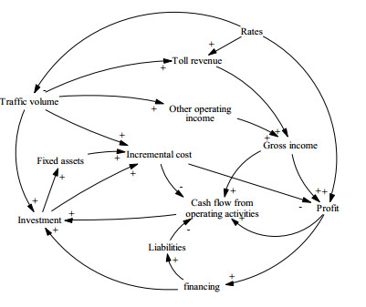
Aiming at the deficiencies presented by the traditional methods of highway project investment evaluation, the proposed highway investment evaluation method was based on system dynamics. First, we constructed an evaluation index system from profitability, solvency, and risk resistance and clarified the positive and negative causality within the investment evaluation system of highway projects; second, we determined the boundaries of the system dynamics model and divided it into six sub-systems, namely, income, cash flow, investment evaluation, profit, cost, investment and financing, and liabilities; and then, we established the system dynamics model of highway investment evaluation based on the sub-systems. The model made up for the limitations of the traditional discounted cash flow method; finally, taking the China's Yunnan Province an Expressway project as an example, using VENSIM software simulation, we get the evaluation results of the system dynamics model and make a comparative analysis with the discounted cash flow method, which showed that the calculation inaccuracies of the NPV and other financial indicators were in a reasonable range, and the evaluation method had strong operability and practicability. The system dynamics investment evaluation model provided a systematic, intuitive, whole-process investment evaluation method, which provided a theoretical basis for the analysis and decision-making of the investment effect of highway projects.
Citation: Yonghua Liu, Hao Deng, Hanqi Gao, Wei Ni. Research on investment evaluation of highway projects based on system dynamics model[J]. AIMS Mathematics, 2024, 9(8): 20326-20349. doi: 10.3934/math.2024989
Aiming at the deficiencies presented by the traditional methods of highway project investment evaluation, the proposed highway investment evaluation method was based on system dynamics. First, we constructed an evaluation index system from profitability, solvency, and risk resistance and clarified the positive and negative causality within the investment evaluation system of highway projects; second, we determined the boundaries of the system dynamics model and divided it into six sub-systems, namely, income, cash flow, investment evaluation, profit, cost, investment and financing, and liabilities; and then, we established the system dynamics model of highway investment evaluation based on the sub-systems. The model made up for the limitations of the traditional discounted cash flow method; finally, taking the China's Yunnan Province an Expressway project as an example, using VENSIM software simulation, we get the evaluation results of the system dynamics model and make a comparative analysis with the discounted cash flow method, which showed that the calculation inaccuracies of the NPV and other financial indicators were in a reasonable range, and the evaluation method had strong operability and practicability. The system dynamics investment evaluation model provided a systematic, intuitive, whole-process investment evaluation method, which provided a theoretical basis for the analysis and decision-making of the investment effect of highway projects.

| [1] | Ministry of Transportation and Communications of the People's Republic of China, National Toll Road Statistics Bulletin 2020, 2021. |
| [2] | Editorial Board of China Journal of Highway, Review of Academic Research on Transportation Engineering in China 2016, China J. Highway, 29 (2016), 1−161. |
| [3] | H. Huang, Discussion of the national toll road statistical bulletin from a financial perspective, Financ. Account., 2019, 77−78. |
| [4] |
Y. H. Liu, R. K. Duan, K. Shen, Q. X. Luan, H. Q. Gao, H. Deng, An investigation into the determinants of satisfaction concerning varied toll policies on highways using the random forest model, AIMS Math., 9 (2024), 4161−4177. https://doi.org/10.3934/math.2024204 doi: 10.3934/math.2024204

|
| [5] |
T. Machiels, T. Compernolle, T. Coppens, Real option applications in megaproject planning: Trends, relevance and research gaps: A literature review, Eur. Plan. Stud., 29 (2021), 446−467. https://doi.org/10.1080/09654313.2020.1742665 doi: 10.1080/09654313.2020.1742665
|
| [6] | X. Y. Cai, G. G. Zhou, Option value analysis of revenue adjustment in operation period of toll road PPP project, Transp. Syst. Eng. Inform., 17 (2017), 7−11. |
| [7] | Y. Wang, L. Ma, J. Bai, Evaluation of financial risk control of large-scale international projects based on neural network, J. Tongji Univ. (Nat. Sci. Edit.), 43 (2015), 1104−1110. |
| [8] | L. Li, An empirical study on the rational selection of comprehensive line solution diagram and calculation period for economic evaluation of construction projects, Pract. Underst. Math., 49 (2019), 9−16. |
| [9] | X. Liu, R. X. Zhou, Y. Zhan, Research on project investment evaluation index based on interval number, J. Beijing Univ. Chem. Technol. (Nat. Sci. Edit.), 44 (2017), 124−127. |
| [10] |
S. P. Shepherd, A review of system dynamics models applied in transportation, Transportmetrica B, 2 (2014), 83−105. https://doi.org/10.1080/21680566.2014.916236 doi: 10.1080/21680566.2014.916236
|
| [11] | Q. N. Liu, Y. W. Wang, M. L. Yao, J. Li, Research on the evolution and simulation of operational risk of PPP project based on system dynamics, J. Eng. Manag., 31 (2017), 57−61. |
| [12] | Z. Y. Zhao, S. Fan, T. Dai, Application of system dynamics model for value-for-money evaluation of PPP projects, J. Huaqiao Univ. (Nat. Sci. Edit.), 41 (2020), 765−771. |
| [13] | C. C. Xue, J. K. Zhou, System dynamics modeling and analysis of PPP project performance–A highway as an example, Financ. Account. Mon., 2019,171−176. |
| [14] |
W. Xu, J. J. Liu, J. M. Li, H. Wang, Q. T. Xiao, A novel hybrid intelligent model for molten iron temperature forecasting based on machine learning, AIMS Math., 9 (2024), 1227−1247. https://doi.org/10.3934/math.2024061 doi: 10.3934/math.2024061
|
| [15] | F. L. Feng, N. Yu, Research on pack back transportation tariff based on system dynamics and logit model, J. Railway Sci. Eng., 15 (2018), 2980−2987. |
| [16] | P. D. Chao, L. Y. Zhou, Y. F. Kang, Simulation analysis of transportation restructuring policy based on system dynamics, Railway Transp. Econ., 46 (2024), 78−89. |
| [17] | Z. W. Wang, Z. Y. Xiang, X. Liu, Research on urban traffic congestion management strategy based on system dynamics model, J. Changsha Univ. Technol. (Nat. Sci. Edit.), 19 (2022), 81−88. |
| [18] |
R. Pokharel, E. J. Miller, K. Chapple, Modeling car dependency and policies towards sustainable mobility: A system dynamics approach, Transport. Res. Part D-Tr. E., 125 (2023), 103978. https://doi.org/10.1016/j.trd.2023.103978 doi: 10.1016/j.trd.2023.103978
|
| [19] |
X. F. Lai, Z. X. Chen, X. Wang, C. H. Chiu, Risk propagation and mitigation mechanisms of disruption and trade risks for a global production network, Transport. Res. E-Log., 170 (2023), 103013. https://doi.org/10.1016/j.tre.2022.103013 doi: 10.1016/j.tre.2022.103013
|
| [20] | Institute of Standards and Quotas, Ministry of Housing and Urban-Rural Development, Institute of Planning and Research, Ministry of Transportation, Methods and parameters of economic evaluation of highway construction projects, China Planning Press, 2010. |
| [21] | Yunnan Province construction cost consulting service standards, T/YNECA 001-2018. |


Figures(22) / Tables(7)

Yonghua Liu, Hao Deng, Hanqi Gao, Wei Ni. Research on investment evaluation of highway projects based on system dynamics model[J]. AIMS Mathematics, 2024, 9(8): 20326-20349. doi: 10.3934/math.2024989


 DownLoad: